Missing Data

MCAR, MAR, and MNAR

Francisco Cardozo, PhD

Welcome, Players

You are data analysts at a dating app. Your company collected data on 1,000 users — height, sex, and whether they completed their full profile.

But something went wrong. The data was incomplete, and now four different versions exist. Only one is the original.

Your goal is to pick a door, analyze the data behind it, and figure out if your data has the truth.

Round 1: Pick a Door

The Four Doors

:::

Behind each door is a version of your dating app data with the same 1,000 users. Three were corrupted by a different unknown force. One was left untouched.

You must choose one door. That’s your dataset.

One door has no missing values at all, you know the truth, so please don’t say your data is complete.

Choose Your Door

Run the following code to randomly select your door:

Write down which door you got. Now let’s see what’s behind it.

Open Your Door

Compute the group means from your dataset:

Write down your results:

Male mean height = ?
Female mean height = ?
How many missing values do you have?

We’ll compare answers across the class in a moment.

Look around the zoom:

Did everyone get the same means?
Did anyone have zero missing values? (don’t tell)

The force behind each door determined whether your results are trustworthy.

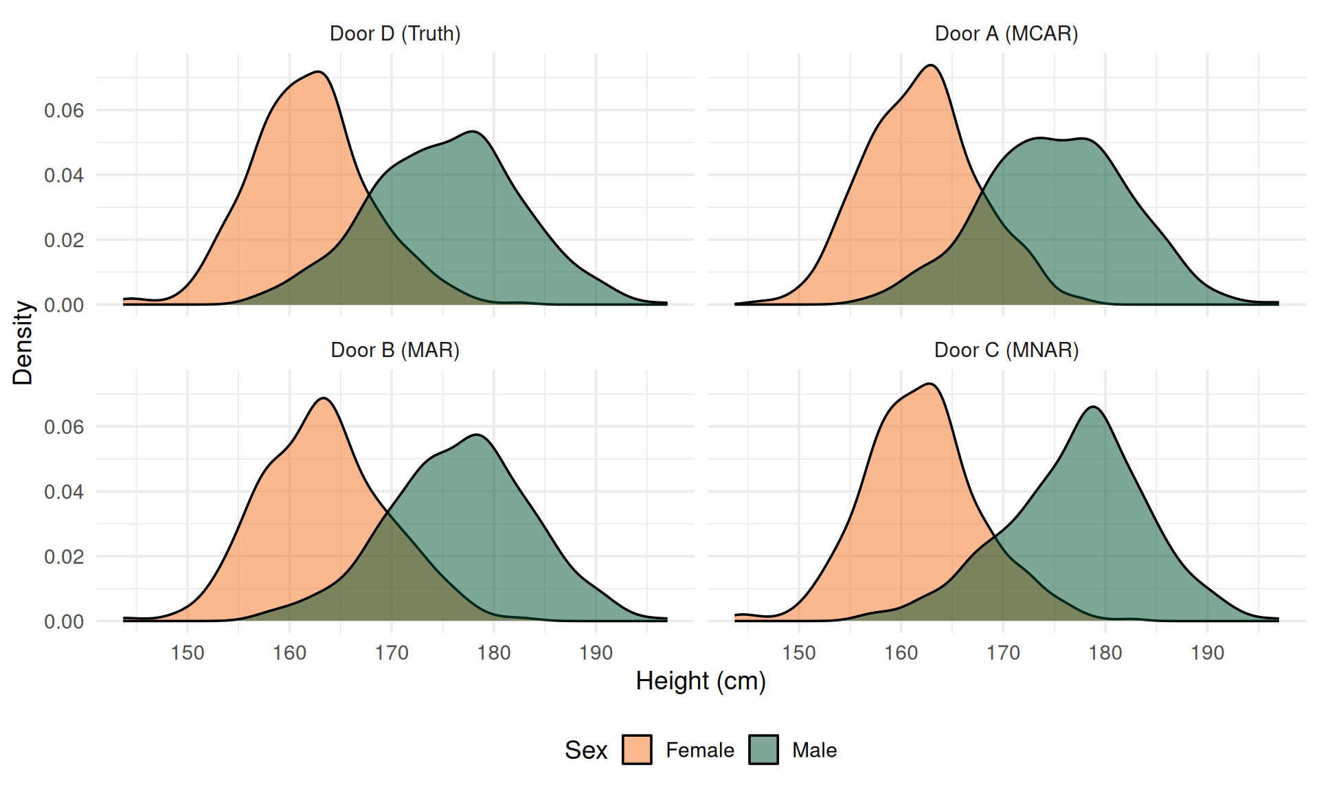
All Four Doors Opened

Let’s see what was behind every door:

Door	Female	Male	Difference (M <U+2212> F)
Door A	162.1	175.2	13.1
Door B	163.4	176.6	13.2
Door C	162.0	177.2	15.2
Door D	161.9	175.3	13.4

Round 2: The Three Forces

Naming the Forces

Rubin [-@rubin1976inference] identified three forces that make data disappear. Each one leaves a different trace and requires a different strategy.

Force (Full Name)	Missingness depends on…
MCAR (Missing Completely At Random)	Nothing — purely random
MAR (Missing At Random)	Observed variables only
MNAR (Missing Not At Random)	The missing values themselves

Learn to recognize each one, then we’ll see which force hit your door.

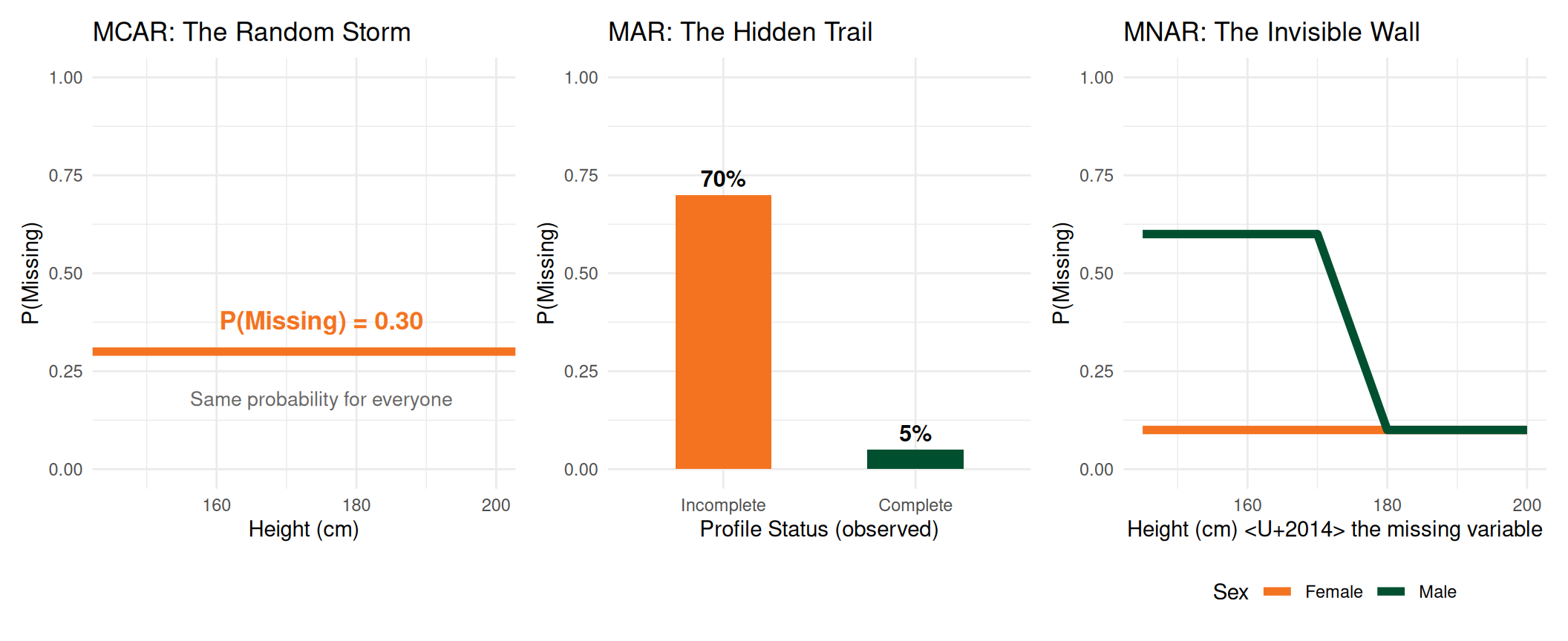
Force 1: MCAR — The Random Storm

Definition: The probability of being missing is unrelated to any variable observed or unobserved.

\[P(R = 1 \mid \text{Sex}, \text{Height}) = P(R = 1)\]

In plain language: This force strikes like lightning completely at random. It doesn’t care who you are or what your height is.

Where you’ll encounter it:

A server crash deletes random records
You don’t ask for height to some users (randomly)
People did not see the height question because it was behind a banner that appears randomly

Good news: Complete-case analysis is unbiased; you lose statistical power.

Planned Missing Data Designs (MCAR by Design)

Researchers sometimes intentionally introduce MCAR to reduce participant burden while preserving statistical power.

Three-form design [@Graham_2006]:

All participants answer a common block (X)
Each participant is randomly assigned two of three additional blocks (A, B, C)
Every item pair appears together in at least one form

Form	Blocks
1	X + A + B
2	X + A + C
3	X + B + C

Why do this?

Cuts survey length by ~33% per participant
Reduces fatigue and careless responding
Missingness is MCAR by construction (random assignment to forms)
MI or FIML recovers full-data estimates with minimal efficiency loss

Other planned designs:

Two-method measurement - expensive gold-standard measure on a random subsample, cheap proxy for everyone
Wave-missing - in longitudinal studies, skip a random subset of participants at certain waves

Force 2: MAR - The Hidden Trail

Definition: The probability of being missing depends on observed data, but not on the missing value itself.

\[P(R = 1 \mid Y_{\text{obs}}, Y_{\text{mis}}) = P(R = 1 \mid Y_{\text{obs}})\]

In plain language: This force follows a trail you can see. If you find the trail, you can undo the damage.

Where you’ll encounter it:

Users who skip their full profile also skip reporting height
Newer users are less likely to fill in optional fields
Users who never upload a photo also leave height blank

Key: Complete-case analysis can be biased, but proper methods (MI, FIML) can correct it if you follow the right trail.

Force 3: MNAR - The Invisible Wall

Definition: The probability of being missing depends on the missing value itself, even after controlling for observed data.

\[P(R = 1 \mid \text{Sex}, \text{Height}) \newline \text{depends directly on height}\]

In plain language: This is the most dangerous force. The data hides because of what it contains. There is no visible trail to follow.

Where you’ll encounter it:

Shorter men don’t report their height on dating apps
High earners refuse to report income
Sickest patients drop out of clinical trials

Warning: No standard method can fully correct this bias. You’ll need sensitivity analysis.

Your Map of the Forces

Feature	MCAR (Random Storm)	MAR (Hidden Trail)	MNAR (Invisible Wall)
Depends on	Nothing	Observed variables	The missing values
Complete-case bias?	No	Yes	Yes
Fixable with MI/FIML?	Yes (N/A)	Yes	Not fully
How common?	Rare	Common	Common
Testable?	Partially	Not definitively	Not definitively

Important

We can never fully verify whether data is MAR or MNAR from the observed data alone. The classification requires substantive reasoning about the data-generating process.

Now, can you match each force to one of the doors?

Round 3: The Reveal

How It Works

I’m going to show you the code used to generate each door’s dataset.

Your job: read the code and tell me what mechanism it is.

Is missingness related to nothing? → MCAR
Is missingness related to an observed variable? → MAR
Is missingness related to the missing value itself? → MNAR

Door A: The Code

data_a <- complete_data |>
    mutate(
        height = ifelse(runif(n()) < 0.40, NA, height)
    )

What do you see?

What determines whether height goes missing?
Does it depend on sex? On height? On profile status?

MCAR — The Random Storm. Every observation has the same 40% chance of being missing. It depends on nothing — pure random chance. The complete cases are a random subset of the data. You lose power, but the truth survives.

Door B: The Code

First, how profile_status was generated:

# Profile completion depends on height
complete_data <- complete_data |>
    mutate(
        p_complete = plogis(
            -0.11 * (height - 170)
        ),
        profile_status = ifelse(
            rbinom(n(), 1, p_complete) == 1,
            "Incomplete",
            "Complete"
        )
    )

Then missingness in height depends on profile_status:

data_b <- complete_data |>
    mutate(
        p_miss = ifelse(profile_status == "Incomplete", 0.70, 0.05),
        height = ifelse(runif(n()) < p_miss, NA, height)
    )

What do you see?

profile_status depends on height; shorter users are less likely to complete their profile
Missingness in height depends on profile_status; not on height directly

MAR - The Hidden Trail. Missingness depends on an observed variable (profile_status). Since shorter users tend to have incomplete profiles (and thus more missing height), the naive group means are biased upward. If we control for profile_status, we can recover the truth.

Door B: Controlling for Profile Status

Try it yourself — estimate the mean height by sex, controlling for profile status:

We can also recover the marginal means using regression + predict:

Door C: The Code

data_c <- complete_data |>
    mutate(
        p_miss = case_when(
            sex == "Female" ~ 0.10,
            height < 170 ~ 0.60,
            height > 180 ~ 0.10,
            TRUE ~ 0.10 + (180 - height) / (180 - 170) * 0.50
        ),
        height = ifelse(runif(n()) < p_miss, NA, height)
    )

What do you see?

What determines whether height goes missing for males?
Can you observe height if it’s the variable that went missing?

MNAR - The Invisible Wall. Among males, missingness depends on height itself; the variable that’s missing. Shorter males have up to 60% chance of being missing. There’s no observed trail to follow.

No standard method can fully correct this.

Door D: The Code

data_d <- complete_data

No problem at all. Door D is the complete, original data; no missing values, no mechanism.

If you chose this door, you had the truth the whole time.

Ground truth: Male = 175.3, Female = 161.9

The Evidence Board

Now let’s compare all four doors against the truth:

Door	Difference	Female	Male
Door D (Truth)	13.4	161.9	175.3
Door A (MCAR)	13.1	162.1	175.2
Door B (MAR)	13.2	163.4	176.6
Door C (MNAR)	15.2	162.0	177.2

Door A (MCAR): close to the truth; random loss, no bias

Door B (MAR): biased; but fixable if we control for profile_status

Door C (MNAR): biased; and not fixable with standard methods

Visualizing the Damage

MAR: Why Is It Biased?

profile_status depends on height. Shorter users are less likely to complete their profile:

complete_data |>
    summarise(
        n = n(),
        mean_height = round(mean(height), 1),
        .by = c(sex, profile_status)
    ) |>
    knitr::kable()

sex	profile_status	n	mean_height
Male	Incomplete	216	172.4
Male	Complete	284	177.5
Female	Incomplete	353	160.8
Female	Complete	147	164.6

Shorter users → incomplete profile → more missing height → observed means are biased upward.

MAR: Following the Trail

But within each profile-status group, missing and observed cases have similar mean heights:

complete_data |>
    mutate(status = ifelse(is.na(data_b$height), "Missing", "Observed")) |>
    summarise(
        n = n(),
        mean_height = round(mean(height), 1),
        .by = c(profile_status, status)
    ) |>
    knitr::kable()

profile_status	status	n	mean_height
Incomplete	Missing	402	164.7
Incomplete	Observed	167	166.5
Complete	Observed	402	173.0
Complete	Missing	29	174.5

This is the signature of MAR. If we include profile_status as an auxiliary variable in MI/FIML, we recover unbiased estimates.

MNAR: Behind the Wall

complete_data |>
    mutate(status = ifelse(is.na(data_c$height), "Missing", "Observed")) |>
    summarise(
        n = n(),
        mean_height = round(mean(height), 1),
        .by = c(profile_status, status)
    ) |>
    knitr::kable()

profile_status	status	n	mean_height
Incomplete	Observed	455	164.9
Incomplete	Missing	114	166.4
Complete	Observed	345	173.5
Complete	Missing	86	171.6

Among males, missing cases are shorter than observed cases. The data disappears because of its own value. No observed variable can explain this; the bias is not fixable with standard methods.

Mapping the Three Forces

The Takeaway

If you ignore the forces:

Group means are biased
Treatment effects are distorted
Confidence intervals miss the truth
p-values are unreliable
Effect sizes are attenuated

Real-world consequences:

Clinical trials underestimate side effects
Surveys underrepresent vulnerable groups
Longitudinal studies suffer from survivor bias
Policy decisions rest on distorted evidence

The method for handling missing data should be informed by the mechanism that generated it. Rubin

Apply to Your Own Research

Consider your own research or a study you’ve recently read:

Which variables might have missing data?
What force (MCAR, MAR, MNAR) is most plausible? Why?
What would happen if you just deleted all incomplete cases?
What observed variables might predict the missingness?

Lessons Learned

Missing data mechanisms matter. They determine whether your results are biased
MCAR (the random storm) is the only safe scenario for complete-case analysis and it’s the rarest
MAR (the hidden trail) can be addressed with proper methods if you follow the right auxiliary variables
MNAR (the invisible wall) is the hardest challenge requires substantive reasoning and sensitivity analysis
Always ask why data is missing, not just how much

Part II: The Toolkit

Equipping Yourself

Now that you can name the forces, you need the right tools to deal with them.

Complete-case analysis: Deleting incomplete cases
Multiple Imputation (MI): Creating plausible completed datasets
Full Information Maximum Likelihood (FIML): Using all available information
Sensitivity analysis: What to do when you suspect MNAR

Multiple Imputation: The Big Idea

Instead of filling in one guess for each missing value, MI creates m plausible completed datasets.

Three steps:

Impute: Generate m completed datasets
Analyze: Fit your model on each one
Pool: Combine with Rubin’s Rules

Each imputed dataset is slightly different, reflecting our uncertainty about what the missing values could have been.

Pooled estimate:

\[\bar{Q} = \frac{1}{m} \sum_{i=1}^{m} \hat{Q}_i\]

Total variance:

\[T = \bar{U} + \left(1 + \frac{1}{m}\right) B\]

Where \(\bar{U}\) = within-imputation variance and \(B\) = between-imputation variance.

MICE: Chained Equations

MICE = Multivariate Imputation by Chained Equations

MICE website

Each variable with missing data gets its own imputation model, using all other variables as predictors.

The algorithm:

Fill in starting values (e.g., random draws from observed)
For each variable with missing data:
- Regress it on all other variables (observed cases)
- Draw imputed values from the predictive distribution
Repeat step 2 for many iterations (cycling)
Store the final imputed dataset
Repeat m times → m complete datasets

Default methods in mice:

Variable Type	Method
Continuous	Predictive mean matching
Binary (2 lev.)	Logistic regression
Nominal (>2 lev.)	Multinomial logit
Ordinal	Proportional odds

A Simulated Clinical Trial

We simulate a randomized trial with 200 participants, two binary predictors, three continuous, and one auxiliary variable (stress):

set.seed(752)
n_mi <- 200

mi_complete <- tibble(
    id = 1:n_mi,
    age = round(rnorm(n_mi, mean = 0, sd = 1), 2),
    female = rbinom(n_mi, 1, 0.55),
    treatment = rbinom(n_mi, 1, 0.5),
    baseline_severity = round(rnorm(n_mi, mean = 0, sd = 1), 2),
    social_support = round(rnorm(n_mi, mean = 0, sd = 1), 2),
    stress = round(rnorm(n_mi, mean = 0, sd = 1), 2),
    outcome = round(
        -0.5 * treatment - 0.3 * age + 0.4 * female +
            0.5 * baseline_severity - 0.3 * social_support +
            0.8 * stress + rnorm(n_mi, 0, 1), 2
    )
)

stress is an auxiliary variable: it affects the outcome but will not be included in the analysis model. It will, however, drive missingness and be available to MICE.

True parameters (analysis model): \(\beta_{\text{trt}} = -0.5\), \(\beta_{\text{age}} = -0.3\), \(\beta_{\text{female}} = 0.4\), \(\beta_{\text{severity}} = 0.5\), \(\beta_{\text{support}} = -0.3\)

Making Data Disappear (MAR)

We corrupt the data with MAR missingness. The probability of being missing depends on observed variables:

mi_data <- mi_complete |>
    mutate(
        # stress (auxiliary) + treatment drive outcome missingness
        p_miss_out = plogis(-0.5 + 1.5 * stress + 1.0 * treatment),
        # Higher age -> more likely to miss social support
        p_miss_ss = plogis(-0.5 + 1.2 * age),
        outcome = ifelse(rbinom(n(), 1, p_miss_out) == 1, NA, outcome),
        social_support = ifelse(rbinom(n(), 1, p_miss_ss) == 1, NA, social_support)
    ) |>
    select(-p_miss_out, -p_miss_ss)

This is MAR because missingness depends only on fully observed variables — stress and treatment drive missingness in outcome, while age drives missingness in social_support. The key twist: stress affects the outcome (\(\beta = 0.8\)) but is not in the analysis model. Complete-case analysis is biased because dropping high-stress treated participants distorts the treatment–outcome relationship (collider bias: treatment \(\rightarrow\) R \(\leftarrow\) stress). MI recovers because stress is included in the imputation model as an auxiliary variable.

Inspect the Damage

mi_data |>
    summarise(across(everything(), ~ sum(is.na(.x)))) |>
    pivot_longer(everything(), names_to = "Variable", values_to = "N_Missing") |>
    mutate(Pct_Missing = round(N_Missing / nrow(mi_data) * 100, 1)) |>
    filter(N_Missing > 0) |>
    knitr::kable()

Variable	N_Missing	Pct_Missing
social_support	95	38
outcome	125	50

md.pattern(mi_data |> select(-id), rotate.names = TRUE)

   age female treatment baseline_severity stress social_support outcome    
78   1      1         1                 1      1              1       1   0
77   1      1         1                 1      1              1       0   1
47   1      1         1                 1      1              0       1   1
48   1      1         1                 1      1              0       0   2
     0      0         0                 0      0             95     125 220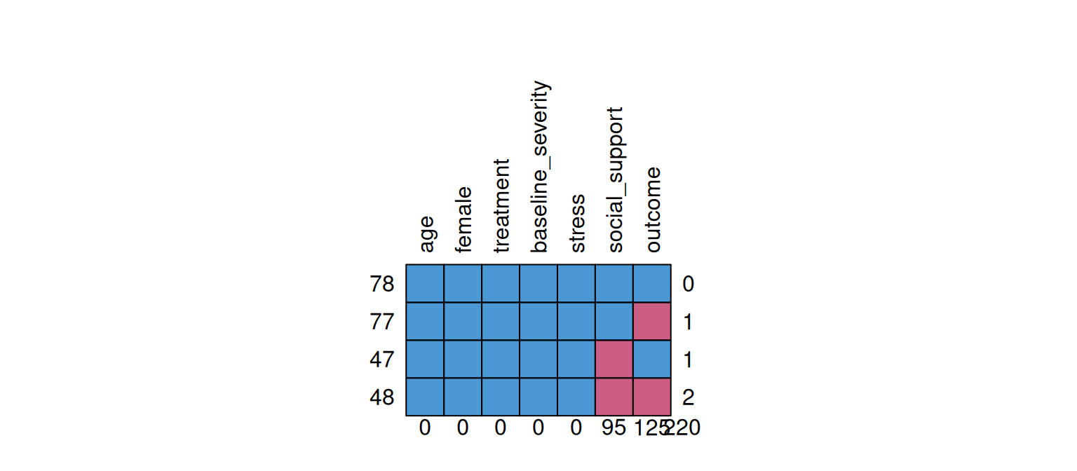

Each row is a pattern (1 = observed, 0 = missing). The numbers show how many cases share each pattern.

Step 1: Run MICE

library(mice)

imp <- mice(
    mi_data |> select(-id),
    m = 5, # number of imputed datasets
    maxit = 20, # iterations per imputation
    seed = 752,
    print = FALSE
)

imp

Class: mids
Number of multiple imputations:  5 
Imputation methods:
              age            female         treatment baseline_severity 
               ""                ""                ""                "" 
   social_support            stress           outcome 
            "pmm"                ""             "pmm" 
PredictorMatrix:
                  age female treatment baseline_severity social_support stress
age                 0      1         1                 1              1      1
female              1      0         1                 1              1      1
treatment           1      1         0                 1              1      1
baseline_severity   1      1         1                 0              1      1
social_support      1      1         1                 1              0      1
stress              1      1         1                 1              1      0
                  outcome
age                     1
female                  1
treatment               1
baseline_severity       1
social_support          1
stress                  1

mice automatically selects predictive mean matching (pmm) for numeric variables. All fully observed variables serve as predictors in each imputation model.

Step 2: Check Convergence

plot(imp)

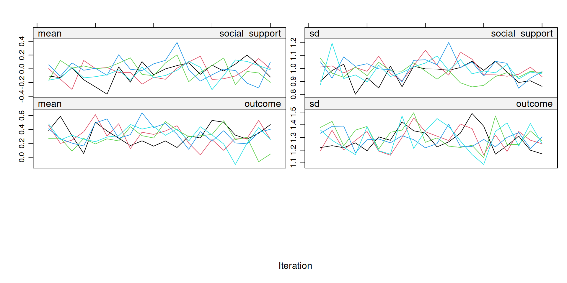
What to look for: The m colored streams should be freely intermixed with no systematic trend. If streams separate or drift upward/downward check the imputation model.

Step 3: Inspect Imputed Values

densityplot(imp)

Blue = observed data distribution. Red lines = imputed distributions (one per imputation). The shapes should be plausible and similar to the observed data, but not necessarily identical.

Step 4: Analyze Each Imputed Dataset

mi_fit <- with(
    imp,
    lm(outcome ~ treatment + age + female +
        baseline_severity + social_support)
)

This fits the same regression model on all 5 imputed datasets. Each produces slightly different estimates because the imputed values differ.

Step 5: Pool with Rubin’s Rules

mi_pooled <- pool(mi_fit)
summary(mi_pooled, conf.int = TRUE) |>
    mutate(across(where(is.numeric), ~ round(.x, 3))) |>
    select(term, estimate, std.error, `2.5 %`, `97.5 %`, p.value) |>
    knitr::kable()

term	estimate	std.error	2.5 %	97.5 %	p.value
(Intercept)	-0.088	0.199	-0.537	0.362	0.670
treatment	-0.522	0.168	-0.861	-0.183	0.003
age	-0.269	0.090	-0.453	-0.084	0.006
female	0.598	0.168	0.262	0.935	0.001
baseline_severity	0.372	0.091	0.187	0.556	0.000
social_support	-0.392	0.093	-0.582	-0.202	0.000

The pooled standard errors incorporate both sampling variability (within) and imputation uncertainty (between).

Complete-Case vs. MI

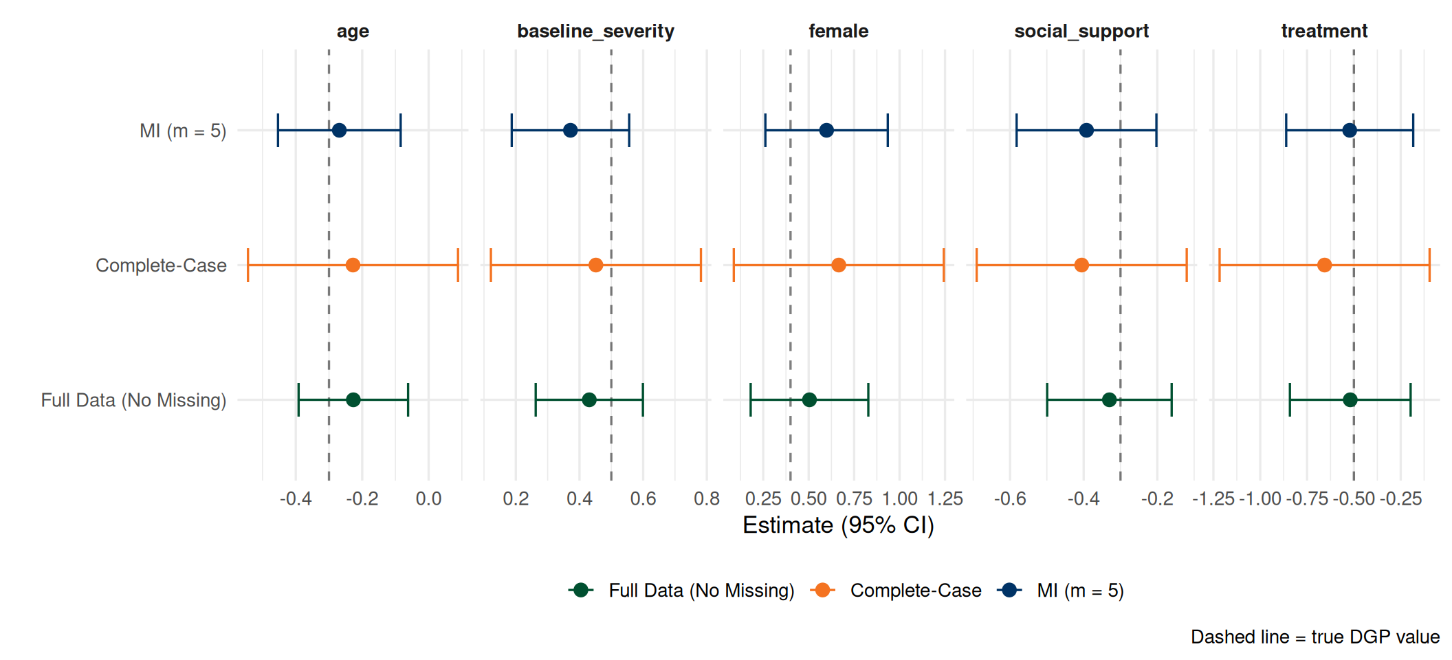
MI recovers estimates close to the full-data truth
MI standard errors properly account for imputation uncertainty (between)
Complete-case discards all partially observed rows, losing efficiency

MI: Practical Guidelines

How many imputations (m)?

Old rule of thumb: m = 5
Other recommendations: m ≥ 20 [@White_2010]
Depends on the fraction of missing information

Include auxiliary variables:

Variables that predict missingness
Variables that correlate with the incomplete variable
Even if they are not in your analysis model

Always check:

Convergence - trace plots should show no trends
Plausibility - imputed distributions should be reasonable
Sensitivity - try different imputation models

Report in your paper:

Number of imputations (m)
Imputation method (e.g., PMM, logistic)
Variables included in the imputation model
Software and version used

The Imputation Model Should Be at Least as General as the Analysis Model

If your analysis includes interactions or nonlinear terms, include them in the imputation model too.

Other MI Packages in R

Beyond mice, several R packages offer alternative approaches to multiple imputation:

Package	Approach	Best For	Link
mice	Chained equations (FCS)	General-purpose, flexible variable-by-variable imputation	CRAN
Amelia	Joint multivariate normal (EMB algorithm)	Large datasets, continuous/normal data, time-series cross-sectional	CRAN
jomo	Joint modelling with random effects	Multilevel / clustered data, mixed variable types	CRAN
missForest	Random forest (single imputation)	Nonlinear relationships, mixed types, no distributional assumptions	CRAN
miceadds	Extensions to mice	Multilevel imputation, two-level models, plausible values	CRAN
mi	Bayesian regression	Diagnostics-rich workflow, automatic transformations	CRAN

How to choose?

Flat data, mixed types \(\rightarrow\) mice (chained equations, most flexible)
Mostly continuous, large N \(\rightarrow\) Amelia (fast joint model, assumes MVN)
Multilevel / clustered \(\rightarrow\) jomo or miceadds (proper random-effects imputation)
Complex nonlinear patterns \(\rightarrow\) missForest (tree-based, but single imputation only)

FIML with lavaan

Full Information Maximum Likelihood (FIML)

FIML estimates model parameters by maximizing the likelihood using all available data, even from incomplete cases.

Unlike MI, FIML does not fill in missing values. Instead, it computes the likelihood for each case based on whatever variables are observed for that case.

Key properties:

Produces unbiased estimates under MAR
Uses all observed information, no cases discarded
Handled natively in lavaan or Mplus with a single argument
No need to create or manage multiple datasets
Equivalent to MI asymptotically (same results, different path)

A 5-Item Anxiety Scale

We simulate a one-factor CFA with 5 items measuring latent anxiety:

library(lavaan)

pop_model <- "
  anxiety =~ 0.80*item1 + 0.70*item2 + 0.60*item3 + 0.75*item4 + 0.65*item5
  anxiety ~~ 1*anxiety
  item1 ~~ 0.36*item1
  item2 ~~ 0.51*item2
  item3 ~~ 0.64*item3
  item4 ~~ 0.4375*item4
  item5 ~~ 0.5775*item5
"

set.seed(2026)
fiml_complete <- simulateData(pop_model, sample.nobs = 2000)

True standardized loadings: \(\lambda_1 = .80\), \(\lambda_2 = .70\), \(\lambda_3 = .60\), \(\lambda_4 = .75\), \(\lambda_5 = .65\)

head(fiml_complete) |>
    mutate(across(everything(), ~ round(.x, 2))) |>
    knitr::kable()

item1	item2	item3	item4	item5
-0.41	-0.87	-0.31	-0.74	0.38
1.14	0.72	0.53	1.12	0.57
0.01	-0.27	0.22	-1.50	1.13
-0.46	1.33	0.53	-0.16	-0.87
0.31	0.71	0.78	0.91	-0.15
2.11	1.88	1.43	1.88	2.37

Survey Fatigue Strikes (MAR)

Participants who score higher on item 1 (more anxious) are more likely to skip later items, a realistic survey fatigue pattern:

fiml_data <- fiml_complete |>
    as_tibble() |>
    mutate(
        # Later items have progressively more missingness
        item3 = ifelse(rbinom(n(), 1, plogis(-2.0 + 0.8 * item1)) == 1, NA, item3),
        item4 = ifelse(rbinom(n(), 1, plogis(-1.5 + 0.8 * item1)) == 1, NA, item4),
        item5 = ifelse(rbinom(n(), 1, plogis(-1.0 + 0.8 * item1)) == 1, NA, item5)
    )

This is MAR: missingness depends on item1 (always observed), not on the missing items themselves.

fiml_data |>
    summarise(across(everything(), ~ sum(is.na(.x)))) |>
    pivot_longer(everything(), names_to = "Item", values_to = "N_Missing") |>
    mutate(Pct = round(N_Missing / nrow(fiml_data) * 100, 1)) |>
    filter(N_Missing > 0) |>
    knitr::kable()

Item	N_Missing	Pct
item3	277	13.9
item4	440	22.0
item5	577	28.8

The CFA Model in lavaan

The model specification is identical for all three analyses. Only the missing argument changes:

cfa_model <- "
  anxiety =~ item1 + item2 + item3 + item4 + item5
"

# 1. Full data (truth <U+2014> no missing values)
fit_true <- cfa(cfa_model, data = fiml_complete)

# 2. Listwise deletion (default)
fit_lw <- cfa(cfa_model, data = fiml_data, missing = "listwise")

# 3. FIML <U+2014> just add one argument
fit_fiml <- cfa(cfa_model, data = fiml_data, missing = "fiml")

That’s It

The only difference is missing = "fiml". lavaan handles everything internally: no imputed datasets, no pooling, no extra steps.

Listwise vs FIML: Factor Loadings

Item	DGP	Full Data	Listwise	FIML	LW (SE)	FIML (SE)
item1	0.80	0.794	0.781	0.798	0.018	0.013
item2	0.70	0.661	0.645	0.667	0.022	0.016
item3	0.60	0.568	0.568	0.565	0.025	0.020
item4	0.75	0.748	0.757	0.754	0.018	0.015
item5	0.65	0.665	0.632	0.650	0.023	0.019

	Full Data	Listwise	FIML
N used	2000	1029	2000

Listwise discards every case with any missing item. FIML uses all 2000 cases.

Listwise vs FIML: Visual Comparison

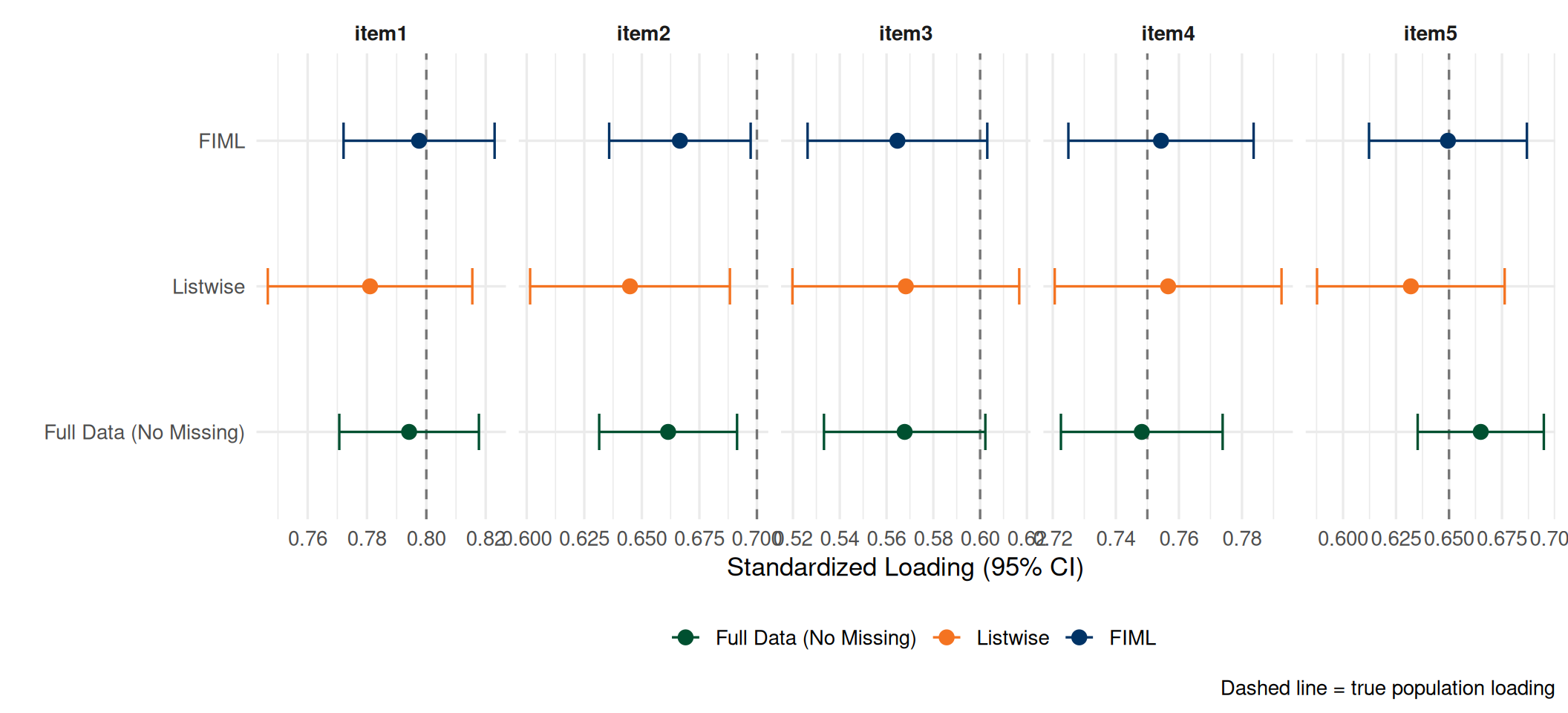
FIML recovers loadings close to the truth — especially for items 3–5 where missingness was highest
Listwise confidence intervals are wider (less efficient) due to reduced sample size

Model Fit: Listwise vs FIML

Index	Full Data	Listwise	FIML
<U+03C7><U+00B2>	6.720	1.704	1.930
df	5.000	5.000	5.000
p-value	0.242	0.888	0.859
CFI	0.999	1.000	1.000
TLI	0.999	1.004	1.002
RMSEA	0.013	0.000	0.000
SRMR	0.008	0.006	0.004

FIML does not improve model fit magically — it provides more accurate estimates of the population parameters by using all available information.

# You can inspect the FIML fit just like any lavaan model
summary(fit_fiml, standardized = TRUE, fit.measures = TRUE)

lavaan 0.6-21 ended normally after 21 iterations

  Estimator                                         ML
  Optimization method                           NLMINB
  Number of model parameters                        15

  Number of observations                          2000
  Number of missing patterns                         8

Model Test User Model:
                                                      
  Test statistic                                 1.930
  Degrees of freedom                                 5
  P-value (Chi-square)                           0.859

Model Test Baseline Model:

  Test statistic                              2494.629
  Degrees of freedom                                10
  P-value                                        0.000

User Model versus Baseline Model:

  Comparative Fit Index (CFI)                    1.000
  Tucker-Lewis Index (TLI)                       1.002
                                                      
  Robust Comparative Fit Index (CFI)             1.000
  Robust Tucker-Lewis Index (TLI)                1.003

Loglikelihood and Information Criteria:

  Loglikelihood user model (H0)             -11008.303
  Loglikelihood unrestricted model (H1)     -11007.338
                                                      
  Akaike (AIC)                               22046.607
  Bayesian (BIC)                             22130.620
  Sample-size adjusted Bayesian (SABIC)      22082.965

Root Mean Square Error of Approximation:

  RMSEA                                          0.000
  90 Percent confidence interval - lower         0.000
  90 Percent confidence interval - upper         0.017
  P-value H_0: RMSEA <= 0.050                    1.000
  P-value H_0: RMSEA >= 0.080                    0.000
                                                      
  Robust RMSEA                                   0.000
  90 Percent confidence interval - lower         0.000
  90 Percent confidence interval - upper         0.019
  P-value H_0: Robust RMSEA <= 0.050             1.000
  P-value H_0: Robust RMSEA >= 0.080             0.000

Standardized Root Mean Square Residual:

  SRMR                                           0.004

Parameter Estimates:

  Standard errors                             Standard
  Information                                 Observed
  Observed information based on                Hessian

Latent Variables:
                   Estimate  Std.Err  z-value  P(>|z|)   Std.lv  Std.all
  anxiety =~                                                            
    item1             1.000                               0.780    0.798
    item2             0.851    0.032   27.009    0.000    0.664    0.667
    item3             0.713    0.033   21.486    0.000    0.556    0.565
    item4             0.984    0.035   28.188    0.000    0.767    0.754
    item5             0.827    0.036   22.899    0.000    0.645    0.650

Intercepts:
                   Estimate  Std.Err  z-value  P(>|z|)   Std.lv  Std.all
   .item1            -0.005    0.022   -0.245    0.807   -0.005   -0.005
   .item2             0.007    0.022    0.313    0.754    0.007    0.007
   .item3             0.010    0.023    0.441    0.659    0.010    0.010
   .item4            -0.004    0.025   -0.146    0.884   -0.004   -0.004
   .item5             0.002    0.025    0.082    0.935    0.002    0.002

Variances:
                   Estimate  Std.Err  z-value  P(>|z|)   Std.lv  Std.all
   .item1             0.348    0.019   18.352    0.000    0.348    0.364
   .item2             0.551    0.022   25.595    0.000    0.551    0.556
   .item3             0.661    0.025   26.203    0.000    0.661    0.681
   .item4             0.446    0.023   19.698    0.000    0.446    0.431
   .item5             0.570    0.025   22.381    0.000    0.570    0.578
    anxiety           0.608    0.032   18.936    0.000    1.000    1.000

FIML vs MI: When is common to use (not a rule)?

FIML:

Your model is a CFA, SEM, or path model
You’re already using lavaan / Mplus
You want a simple, single-step solution
You prefer not to manage multiple datasets

MI:

Your analysis is not SEM-based (e.g., regression, ANOVA, mixed models)
You need to use software that doesn’t support FIML
You want to include many auxiliary variables flexibly
You need to do sensitivity analyses with different imputation models

Important

Both MI and FIML assume MAR. If you suspect MNAR, you need sensitivity analysis, neither method alone can save you.

Wrapping Up: Your Complete Toolkit

Method	When to Use	Assumption	Bias?
Complete-case	Quick look, MCAR only	MCAR	No (under MCAR)
MI (MICE)	Any model, any software	MAR	No (under MAR)
FIML	CFA / SEM models	MAR	No (under MAR)
Sensitivity	When MNAR is suspected	MNAR	Depends

Your workflow:

Diagnose Why is data missing? (MCAR / MAR / MNAR)
Choose Pick the right tool for your model and mechanism
Check Convergence, plausibility, sensitivity
Report Be transparent about what you did and why

References

Little, R. J. A., & Rubin, D. B. (2002). Statistical Analysis with Missing Data (2nd ed.). Wiley.
Rubin, D. B. (1976). Inference and missing data. Biometrika, 63(3), 581–592.
Enders, C. K. (2010). Applied Missing Data Analysis. Guilford Press.
Schafer, J. L., & Graham, J. W. (2002). Missing data: Our view of the state of the art. Psychological Methods, 7(2), 147–177.
van Buuren, S., & Groothuis-Oudshoorn, K. (2011). mice: Multivariate Imputation by Chained Equations in R. Journal of Statistical Software, 45(3), 1–67.
Rosseel, Y. (2012). lavaan: An R package for structural equation modeling. Journal of Statistical Software, 48(2), 1–36.
White, I. R., Royston, P., & Wood, A. M. (2011). Multiple imputation using chained equations: Issues and guidance for practice. Statistics in Medicine, 30(4), 377–399.

Missing Data

Welcome, Players

Round 1: Pick a Door

The Four Doors

Choose Your Door

Open Your Door

Look around the zoom:

All Four Doors Opened

Round 2: The Three Forces

Naming the Forces

Force 1: MCAR — The Random Storm

Planned Missing Data Designs (MCAR by Design)

Force 2: MAR - The Hidden Trail

Force 3: MNAR - The Invisible Wall

Your Map of the Forces

Round 3: The Reveal

How It Works

Door A: The Code

Door B: The Code

Door B: Controlling for Profile Status

Door C: The Code

Door D: The Code

The Evidence Board

Visualizing the Damage

MAR: Why Is It Biased?

MAR: Following the Trail

MNAR: Behind the Wall

Mapping the Three Forces

The Takeaway

Apply to Your Own Research

Lessons Learned

Part II: The Toolkit

Equipping Yourself

Multiple Imputation: The Big Idea

MICE: Chained Equations

A Simulated Clinical Trial

Making Data Disappear (MAR)

Inspect the Damage

Step 1: Run MICE

Step 2: Check Convergence

Step 3: Inspect Imputed Values

Step 4: Analyze Each Imputed Dataset

Step 5: Pool with Rubin’s Rules

Complete-Case vs. MI

MI: Practical Guidelines

Other MI Packages in R

FIML with lavaan

Full Information Maximum Likelihood (FIML)

A 5-Item Anxiety Scale

Survey Fatigue Strikes (MAR)

The CFA Model in lavaan

Listwise vs FIML: Factor Loadings

Listwise vs FIML: Visual Comparison

Model Fit: Listwise vs FIML

FIML vs MI: When is common to use (not a rule)?

Wrapping Up: Your Complete Toolkit

References

Questions?