[1] 0.2385088Multilevel Models
From Independence Violations to Mixed-Effects and GEE
Francisco Cardozo, PhD
Part I: Independence of Observations
A Fundamental Assumption
Most classical statistical methods, including t-tests, ANOVA, and OLS regression, share a core assumption:
\[\text{Cov}(e_i, e_j) = 0 \quad \text{for all } i \neq j\]
Each observation’s residual is unrelated to every other observation’s residual.
This means that knowing one person’s score tells you nothing about another person’s score, beyond what the model already predicts.
Why Does This Matter?
When independence holds:
- Standard errors are correct
- Confidence intervals have proper coverage
- p-values reflect the true Type I error rate
- Statistical tests have the expected power
When it doesn’t, all of these break down.
What Independence Looks Like
Consider a simple study: we measure depression scores in 100 individuals randomly sampled from the population.
The correlation between arbitrary pairs is near zero, and each score is independent of every other.
The Independence Assumption in Practice
Independence is plausible when:
- Participants are randomly and independently sampled
- No participant influences another
- No shared environment or grouping structure
- No repeated measurements on the same unit
Independence is violated when:
- Students are nested within classrooms
- Patients are treated by the same therapist
- Observations are repeated over time on the same person
- Family members share a household
- Employees work in the same organization
In the social, behavioral, and health sciences, truly independent observations are the exception, not the rule.
Part II: Understanding Clustered Data
What Is Clustered Data?
Clustered data arises when observations are grouped into higher-level units:
| Level 1 (Observations) | Level 2 (Clusters) |
|---|---|
| Students | Schools |
| Patients | Clinics |
| Time points | Individuals |
| Employees | Organizations |
| Trials | Participants |
Observations within the same cluster tend to be more similar to each other than observations from different clusters.
This within-cluster similarity is quantified by the Intraclass Correlation Coefficient (ICC):
\[\rho = \frac{\sigma^2_{\text{between}}}{\sigma^2_{\text{between}} + \sigma^2_{\text{within}}}\]
- \(\rho = 0\): no clustering effect (observations are independent)
- \(\rho = 1\): all variation is between clusters (observations within a cluster are identical)
Simulating Clustered Data
Let’s create data where students are nested within 20 schools, with 10 students per school:
set.seed(2026)
n_schools <- 20
n_students <- 10

school_effects <- rnorm(n_schools, mean = 0, sd = 5)

clustered_data <- tibble(
    school = rep(1:n_schools, each = n_students),
    school_effect = rep(school_effects, each = n_students),
    student_error = rnorm(n_schools * n_students, mean = 0, sd = 3),
    score = 50 + school_effect + student_error
)
The school effect (\(\sigma^2_b = 25\)) creates dependence among students within the same school. The student error (\(\sigma^2_w = 9\)) represents individual variation.
True ICC = \(25 / (25 + 9)\) = 0.735
Visualizing the Clustering
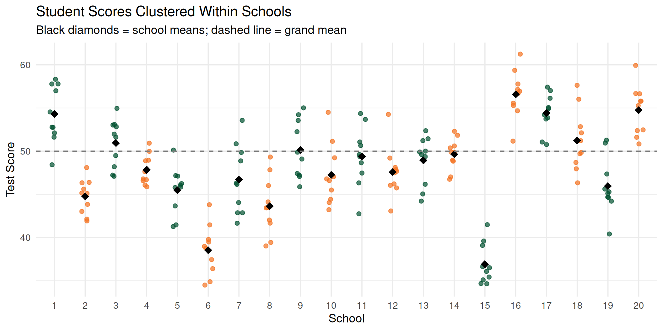
Students within the same school cluster around their school mean. Ignoring this structure leads to incorrect inferences.
Why Ignoring Clustering Is Dangerous
The core problem: Standard errors depend on sample size. The more independent observations you have, the smaller the SE.
But when data is clustered, observations within the same cluster carry redundant information. If two students in the same school score similarly because of shared environment, counting them as two fully independent data points overstates how much information you actually have.
OLS doesn’t know about clustering, so it thinks:
“I have 200 independent observations, so my SE should be small!”
But the real information content is less than 200. It’s as if you had fewer observations.
The Design Effect tells you how much redundancy exists:
\[\text{DEFF} = 1 + (m - 1) \times \rho\]
Where \(m\) = cluster size and \(\rho\) = ICC.
Example: 10 schools × 30 students, ICC = 0.25
\[\text{DEFF} = 1 + (30 - 1)(0.25) = 8.25\]
\[N_{\text{effective}} = \frac{300}{8.25} \approx 36\]
OLS thinks you have 300 observations. You effectively have 36.
Since \(SE \propto 1/\sqrt{N}\), the underestimation factor is:
\[\frac{SE_{\text{correct}}}{SE_{\text{OLS}}} = \sqrt{\frac{N}{N_{\text{eff}}}} = \sqrt{\text{DEFF}} = \sqrt{8.25} \approx 2.9\]
The OLS standard error is 2.9× too small. That means confidence intervals are too narrow, p-values are too small, and you reject the null far more often than 5% even when the null is true.
A Demonstration: Ignoring Clustering
Let’s create a dataset where there is no treatment effect (\(\beta_1 = 0\)) but observations are clustered within 10 schools (30 students each, \(N\) = 300). Treatment is assigned at the school level (5 schools per condition). We set the ICC to 0.25, the same value from the DEFF example:
set.seed(2026)
n_schools_demo <- 10
n_per_school <- 30
sigma_u_demo <- sqrt(0.25) # school SD → ICC = 0.25/(0.25+0.75) = 0.25
sigma_e_demo <- sqrt(0.75) # student SD

school_intercepts <- rnorm(n_schools_demo, 0, sd = sigma_u_demo)

demo_data <- tibble(
    school = rep(1:n_schools_demo, each = n_per_school),
    treatment = rep(c(0, 1), each = n_schools_demo / 2 * n_per_school),
    school_effect = rep(school_intercepts, each = n_per_school),
    y = 50 +
        0 * treatment +
        school_effect +
        rnorm(n_schools_demo * n_per_school, 0, sd = sigma_e_demo)
)
The true treatment effect is exactly zero. Any “significant” result is a false positive.
Where Does the False Positive Come From?
Let’s look at the school means by treatment group:
| school | school_mean | treatment |
|---|---|---|
| 1 | 50.38 | 0 |
| 2 | 49.20 | 0 |
| 3 | 50.09 | 0 |
| 4 | 50.02 | 0 |
| 5 | 49.86 | 0 |
| 6 | 48.82 | 1 |
| 7 | 49.77 | 1 |
| 8 | 49.52 | 1 |
| 9 | 50.12 | 1 |
| 10 | 49.84 | 1 |
| treatment | group_mean |
|---|---|
| 0 | 49.91 |
| 1 | 49.61 |
The group means differ, not because treatment works, but because different schools were assigned to each group, and schools have different baseline levels (the random intercepts).
The Source of the False Positive
- Each school got a random intercept (\(u_{0j}\)) by chance
- Treatment was assigned at the school level
- The 5 “treatment” schools happened to draw different intercepts than the 5 “control” schools
- OLS sees 300 data points and computes a tiny SE, small enough that this chance difference looks “significant”
- The mixed model recognizes these are only 10 schools, gives a larger SE, and correctly fails to reject
OLS vs. Mixed Model: Same Data, Different Conclusions
Naive OLS (ignores clustering):
What Just Happened?
ols_se <- summary(ols_fit)$coefficients["treatment", "Std. Error"]
mix_se <- summary(mixed_fit)$coefficients["treatment", "Std. Error"]

tibble(
    Model = c("OLS (naive)", "Mixed model"),
    Estimate = c(coef(ols_fit)["treatment"], fixef(mixed_fit)["treatment"]),
    `Std. Error` = c(ols_se, mix_se),
    `SE Ratio` = c(1, mix_se / ols_se)
) |>
    mutate(across(where(is.numeric), ~ round(.x, 3))) |>
kable()| Model | Estimate | Std. Error | SE Ratio |
|---|---|---|---|
| OLS (naive) | -0.296 | 0.105 | 1.000 |
| Mixed model | -0.296 | 0.295 | 2.798 |
The point estimates are similar. Both models estimate approximately the same treatment effect.
But the standard errors are dramatically different. The mixed model’s SE is roughly 2.8x larger than OLS.
Does this match the DEFF formula? We simulated with \(\sigma^2_u = 0.25\) and \(\sigma^2_e = 0.75\), so the true ICC = 0.25, and cluster size \(m\) = 30, the same values from the earlier slide:
DEFF = 8.25
√DEFF = 2.87
Observed SE ratio = 2.8
The observed ratio is close to \(\sqrt{\text{DEFF}} = \sqrt{8.25} \approx 2.9\). The formula and the model agree.
How Often Does OLS Get It Wrong?
Let’s repeat this 1,000 times. Each time the true effect is zero, and we count how often each method falsely rejects:
set.seed(2026)
n_sims <- 1000

sim_results <- map_dfr(1:n_sims, \(i) {
    school_eff <- rnorm(n_schools_demo, 0, sd = sigma_u_demo)
    d <- tibble(
        school = rep(1:n_schools_demo, each = n_per_school),
        treatment = rep(c(0, 1), each = n_schools_demo / 2 * n_per_school),
        y = 50 +
            rep(school_eff, each = n_per_school) +
            rnorm(n_schools_demo * n_per_school, 0, sd = sigma_e_demo)
    )
    p_ols <- summary(lm(y ~ treatment, data = d))$coefficients[2, 4]
    p_mix <- summary(lmer(y ~ treatment + (1 | school), data = d))$coefficients[
        2,
        5
    ]
    tibble(p_ols, p_mix)
})| Model | Type I Error Rate | Expected |
|---|---|---|
| OLS (naive) | 0.500 | 0.05 |
| Mixed model | 0.045 | 0.05 |
OLS falsely rejects far more than 5% of the time. The mixed model stays close to the nominal rate.
Visualizing the Inflation
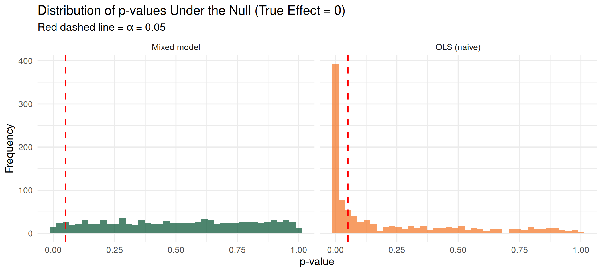
Under the null, p-values should be uniformly distributed. OLS produces a spike near zero (too many false positives). The mixed model produces the expected uniform distribution.
The Core Insight
What standard regression assumes:
\[y_i = \beta_0 + \beta_1 x_i + e_i\]
All observations are exchangeable. The only source of variation is individual-level error \(e_i\).
What the data actually looks like:
\[y_{ij} = \beta_0 + \beta_1 x_{ij} + u_j + e_{ij}\]
Observations \(i\) are nested within clusters \(j\). There are two sources of variation:
- \(u_j\): cluster-level variation (between)
- \(e_{ij}\): individual-level variation (within)
We need models that acknowledge this hierarchical structure. That’s where mixed-effects models come in.
Part III: Mixed-Effects Models
The Mixed-Effects Framework
A mixed-effects model (also called a multilevel, hierarchical, or random-effects model) contains two types of effects:
- Fixed effects: parameters that are constant across all clusters (like a regular regression coefficient)
- Random effects: parameters that vary across clusters, drawn from a distribution
The simplest mixed model adds a random intercept:
\[y_{ij} = \underbrace{\beta_0 + \beta_1 x_{ij}}_{\text{fixed}} + \underbrace{u_{0j}}_{\text{random}} + e_{ij}\]
where \(u_{0j} \sim N(0, \sigma^2_u)\) and \(e_{ij} \sim N(0, \sigma^2_e)\)
Intuition
Think of the random intercept as saying: each cluster has its own baseline level, and these baselines are drawn from a normal distribution.
- A community with \(u_{0j} > 0\) has higher-than-average risk
- A community with \(u_{0j} < 0\) has lower-than-average risk
- The variance \(\sigma^2_u\) tells us how much clusters differ
Let’s See It with Data
Imagine a prevention study: 5 communities each have 4 schools that implement a substance use prevention program. We measure the risk behavior score at each school after the program.
prevention_data <- tibble(
    community = rep(paste("Community", LETTERS[1:5]), each = 4),
    school = 1:20,
    risk_score = c(
        42,
        47,
        39,
        44, # Community A - cluster mean ≈ 43
        31,
        28,
        35,
        30, # Community B - cluster mean ≈ 31
        55,
        58,
        51,
        60, # Community C - cluster mean ≈ 56
        38,
        41,
        36,
        33, # Community D - cluster mean ≈ 37
        48,
        52,
        45,
        51 # Community E - cluster mean ≈ 49
    )
)
The scores within the same community are more similar to each other than scores from different communities. That’s the clustering.
Look at the Data
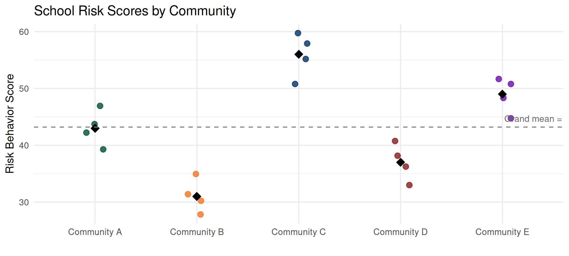
The black diamonds are community means. Some communities’ schools report higher risk, others lower. That between-community variation is what a random effect captures.
Two Sources of Variation
Every school’s score can be decomposed:
\[\text{risk}_{ij} = \underbrace{\text{grand mean}}_{\beta_0} + \underbrace{\text{community deviation}}_{{u_{0j}}} + \underbrace{\text{school deviation}}_{e_{ij}}\]
Let’s compute this by hand:
prevention_summary <- prevention_data |>
    mutate(grand_mean = mean(risk_score)) |>
    summarise(
        community_mean = mean(risk_score),
        grand_mean = first(grand_mean),
        community_deviation = community_mean - grand_mean,
        n = n(),
        .by = community
    )

prevention_summary |>
    mutate(across(where(is.numeric), ~ round(.x, 1))) |>
kable()| community | community_mean | grand_mean | community_deviation | n |
|---|---|---|---|---|
| Community A | 43 | 43.2 | -0.2 | 4 |
| Community B | 31 | 43.2 | -12.2 | 4 |
| Community C | 56 | 43.2 | 12.8 | 4 |
| Community D | 37 | 43.2 | -6.2 | 4 |
| Community E | 49 | 43.2 | 5.8 | 4 |
The community deviation (\(u_{0j}\)) is how far each community’s mean is from the grand mean. This is the random effect.
Partitioning the Variance
Now let’s quantify the two variance components:
grand_mean <- mean(prevention_data$risk_score)

between_variance <- prevention_data |>
    summarise(community_mean = mean(risk_score), .by = community) |>
    summarise(var_between = var(community_mean)) |>
    pull(var_between)

within_variance <- prevention_data |>
    mutate(community_mean = mean(risk_score), .by = community) |>
    mutate(deviation = risk_score - community_mean) |>
    summarise(var_within = var(deviation)) |>
    pull(var_within)

tibble(
    Component = c(
        "Between communities (σ²_u)",
        "Within communities (σ²_e)",
        "Total"
    ),
    Variance = c(
        between_variance,
        within_variance,
        between_variance + within_variance
    )
) |>
    mutate(
        Percent = round(
            Variance / sum(head(Variance, 2)) * c(1, 1, 1) * 100,
            1
        ),
        Variance = round(Variance, 2)
    ) |>
kable()| Component | Variance | Percent |
|---|---|---|
| Between communities (σ²_u) | 96.20 | 91.5 |
| Within communities (σ²_e) | 8.95 | 8.5 |
| Total | 105.15 | 100.0 |
Most of the variance is between communities. Schools within the same community have similar risk levels.
Fitting the Empty Model
Now let’s let lmer estimate these variance components formally:
Linear mixed model fit by REML. t-tests use Satterthwaite's method [
lmerModLmerTest]
Formula: risk_score ~ 1 + (1 | community)
   Data: prevention_data

REML criterion at convergence: 117.1

Scaled residuals:
    Min      1Q  Median      3Q     Max
-1.3732 -0.5523 -0.1459  0.7650  1.3002

Random effects:
 Groups    Name        Variance Std.Dev.
 community (Intercept) 93.37    9.663
 Residual              11.33    3.367
Number of obs: 20, groups:  community, 5

Fixed effects:
            Estimate Std. Error     df t value Pr(>|t|)
(Intercept)   43.200      4.386  4.000   9.849 0.000596 ***
---
Signif. codes:  0 '***' 0.001 '**' 0.01 '*' 0.05 '.' 0.1 ' ' 1
Reading the Output
The model estimated:
| Component | Variance | SD |
|---|---|---|
| Between (σ²_u) | 93.37 | 9.66 |
| Within (σ²_e) | 11.33 | 3.37 |
- \(\hat{\sigma}^2_u\) = 93.37, variance between communities
- \(\hat{\sigma}^2_e\) = 11.33, variance within communities (between schools in the same community)
The fixed effect:
This is the grand mean, the overall average risk score across all communities and schools.
The random effects (BLUPs):
            (Intercept)
Community A       -0.19
Community B      -11.84
Community C       12.42
Community D       -6.02
Community E        5.63
These are the estimated \(u_{0j}\), each community’s deviation from the grand mean.
From Variance Components to the ICC
The Intraclass Correlation Coefficient is simply the proportion of total variance that is between clusters:
\[\text{ICC} = \frac{\sigma^2_u}{\sigma^2_u + \sigma^2_e} = \frac{\text{between-community variance}}{\text{total variance}}\]
What this means:
- 89% of the total variation in risk scores is due to differences between communities
- 11% is due to differences between schools within the same community
- Schools in the same community have much more similar risk levels than schools in different communities
The ICC Is the Reason We Need Mixed Models
If ICC = 0, there is no clustering; all communities have similar risk levels and OLS is fine.
As ICC increases, observations within clusters become more dependent, and ignoring this leads to underestimated standard errors and inflated Type I error.
ICC, R², and the F-Ratio: One Family
The ICC might look new, but it belongs to a family of statistics you already know, all based on the same idea: partitioning variance.
| Statistic | Question It Answers |
|---|---|
| R² | How much variance in \(y\) is explained by the predictor \(x\)? |
| F-ratio | Is the variance between groups large relative to the variance within groups? |
| ICC | What proportion of total variance is between clusters? |
All three decompose total variance into “signal” and “noise”; they just define those terms differently.
The Common Thread
\[\text{Total Variance} = \text{Explained (between)} + \text{Unexplained (within)}\]
- R² = \(\frac{SS_{\text{regression}}}{SS_{\text{total}}}\), proportion explained by predictors
- F = \(\frac{MS_{\text{between}}}{MS_{\text{within}}}\), ratio of between to within
- ICC = \(\frac{\sigma^2_u}{\sigma^2_u + \sigma^2_e}\), proportion due to clustering
They are different lenses on the same fundamental operation.
Connecting Them with Our Data
Let’s compute all three on the prevention data and see how they relate:
            Df Sum Sq Mean Sq F value    Pr(>F)
community    4 1539.2  384.80  33.953 2.355e-07 ***
Residuals   15  170.0   11.33
---
Signif. codes:  0 '***' 0.001 '**' 0.01 '*' 0.05 '.' 0.1 ' ' 1
f_ratio <- anova_table$`F value`[1]
r_squared <- anova_table$`Sum Sq`[1] / sum(anova_table$`Sum Sq`)
tibble(
Statistic = c("R² (from ANOVA)", "F-ratio", "ICC (from lmer)"),
Value = round(c(r_squared, f_ratio, icc_value), 3),
Interpretation = c(
paste0(
round(r_squared * 100, 1),
"% of variance explained by community"
),
paste0(
"Between-group MS is ",
round(f_ratio, 1),
"x the within-group MS"
),
paste0(
round(icc_value * 100, 1),
"% of variance is between communities"
)
)
) |>
kable()| Statistic | Value | Interpretation |
|---|---|---|
| R² (from ANOVA) | 0.901 | 90.1% of variance explained by community |
| F-ratio | 33.953 | Between-group MS is 34x the within-group MS |
| ICC (from lmer) | 0.892 | 89.2% of variance is between communities |
How They Relate
R² and ICC ask a similar question, what proportion of variance is between groups, but they answer it differently.
R² uses raw sums of squares:
\[R^2 = \frac{SS_{\text{between}}}{SS_{\text{total}}}\]
The problem: \(SS_{\text{between}}\) reflects the observed spread of group means, but those means are noisy estimates. With only 4 schools per community, each mean carries sampling error. So \(SS_{\text{between}}\) is inflated by within-group noise leaking into the group means.
ICC uses REML variance components that correct for this:
\[\hat{\sigma}^2_u = \frac{MS_{\text{between}} - MS_{\text{within}}}{n_j}\]
It subtracts out the within-group mean square before computing between-cluster variance. R² tends to overestimate the between-cluster proportion, especially with small clusters. As cluster size grows, the correction becomes negligible and R² \(\to\) ICC.
The F-ratio tells the same story as a ratio instead of a proportion:
- \(F \approx 1\): between-group variance \(\approx\) within-group variance → no clustering
- \(F \gg 1\): between-group variance dominates → strong clustering
You can recover the ICC from the F-ratio of a one-way ANOVA:
\[\text{ICC} \approx \frac{F - 1}{F - 1 + n_j}\]
where \(n_j\) is the cluster size.
| R² (ANOVA) | ICC (lmer) | |
|---|---|---|
| Uses | Raw sums of squares | REML variance components |
| Corrects for | Nothing | Sampling error in group means |
| Type | Sample descriptive | Population parameter estimate |
| Bias | Overestimates with small clusters | Unbiased |
The Bottom Line
If you understand R² and the F-ratio, you already understand the ICC. It’s the same variance decomposition; the ICC just does it more carefully by accounting for the fact that group means are themselves estimated with error.
Putting It All Together
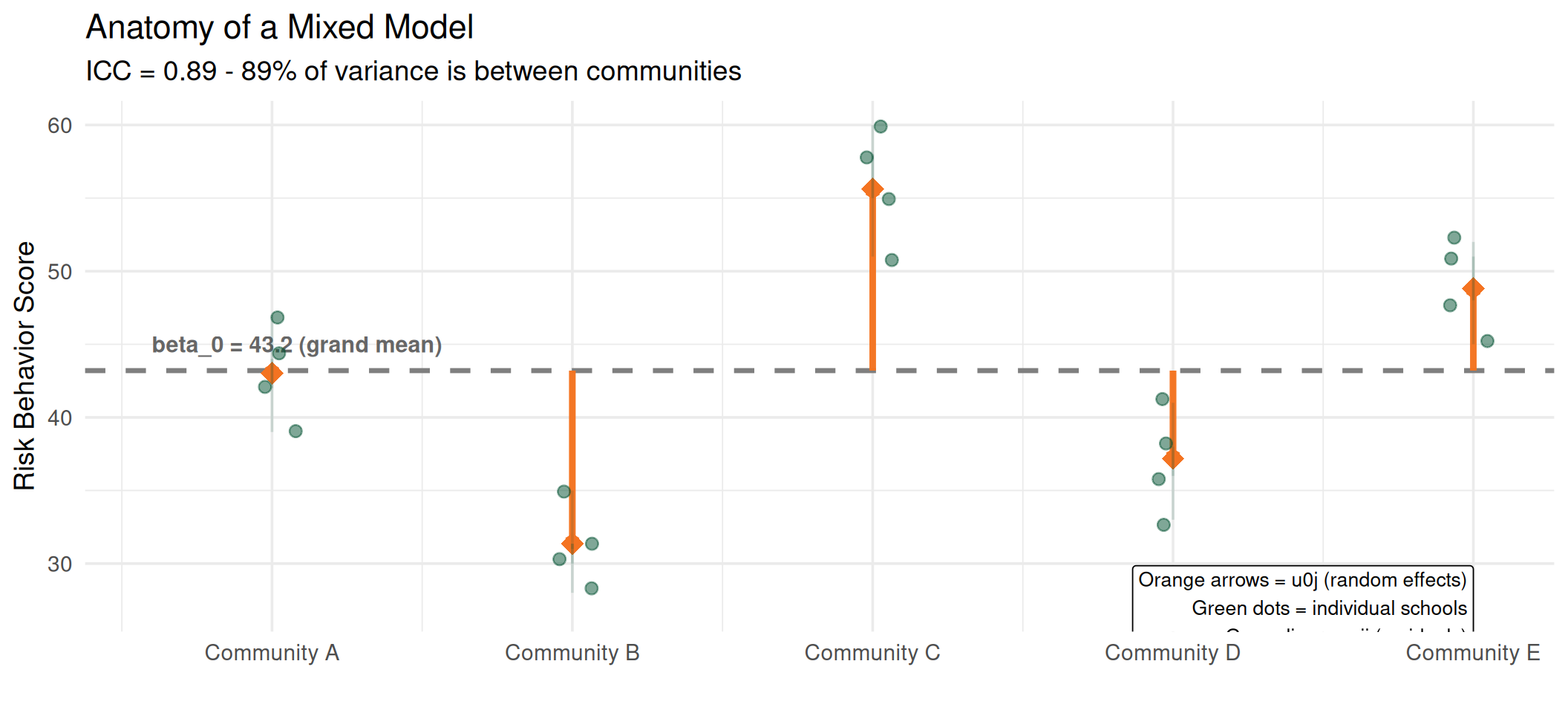
The grand mean (\(\beta_0\)) is the fixed effect. The orange arrows (\(u_{0j}\)) are the random effects, showing how far each community deviates. The green lines (\(e_{ij}\)) are individual school residuals.
What Are Random Effects?
Now we can answer precisely:
Fixed effects answer: What is the average effect of \(x\) on \(y\) across all clusters?
Random effects answer: How much do clusters vary around that average?
| Fixed Effects | Random Effects | |
|---|---|---|
| Estimated | Point estimates (\(\hat{\beta}\)) | Variance components (\(\hat{\sigma}^2_u\)) |
| Interpretation | Average relationship | Variability across clusters |
| Inference | About the specific predictors | About the population of clusters |
| Assumption | Same for all clusters | Drawn from a distribution |
When to Use Random Effects
Use a random effect when:
- Your clusters are a sample from a larger population (schools, therapists, participants)
- You want to generalize beyond the observed clusters
- You want to account for within-cluster correlation
- You have enough clusters (typically \(\geq\) 20)
Use fixed effects for clusters when:
- You have a small, exhaustive set (e.g., 3 treatment conditions)
- You are interested in the specific cluster differences
Fixed-Effects vs. Mixed Models: Generalizability
There is an important distinction between treating clusters as fixed versus random that goes beyond estimation; it changes what your results mean.
Fixed-effects model (clusters as dummies):
\[y_{ij} = \beta_0 + \beta_1 x_{ij} + \gamma_2 D_{2j} + \gamma_3 D_{3j} + \cdots + e_{ij}\]
- Estimates a separate parameter for each cluster
- Conclusions are limited to these specific clusters
- No distributional assumption about cluster effects
- Cannot predict outcomes for a new cluster
“Community B’s schools score 12 points lower than Community A’s.”
Mixed model (clusters as random):
\[y_{ij} = \beta_0 + \beta_1 x_{ij} + u_{0j} + e_{ij}, \quad u_{0j} \sim N(0, \sigma^2_u)\]
- Estimates a variance component, how much clusters vary in general
- Conclusions generalize to the population of clusters
- Assumes cluster effects follow a distribution
- Can predict outcomes for a new, unobserved cluster (via the distribution)
“Communities vary with \(\sigma_u\) = 10; a new community’s schools will likely fall within that range.”
The Generalizability Trade-Off
| Fixed Effects | Mixed (Random) Effects | |
|---|---|---|
| Clusters are | Specific, known, exhaustive | A sample from a larger population |
| Inference to | Only these clusters | The population of all clusters |
| External validity | Low, results are cluster-specific | High, results generalize |
| New cluster? | Cannot predict | Can predict (from \(\hat{\sigma}^2_u\)) |
| Example | 3 specific drug doses | 30 schools sampled from a district |
Why This Matters
Suppose you study the effect of a tutoring program across 25 schools.
Fixed-effects approach: “The program worked in School 3 and School 17, but not in School 8.” Your conclusions apply to these 25 schools only.
Mixed-effects approach: “The program increases scores by 5 points on average, with \(\sigma_u\) = 3 across schools.” Your conclusions apply to any similar school, including ones you didn’t study.
If you want to inform policy, whether to scale the program to new schools, the mixed model gives you the evidence you need.
When Fixed Effects Make Sense
Fixed-effects models for clusters are not wrong; they answer a different question. Use them when:
- You have a small, exhaustive set of clusters (e.g., 2 treatment conditions, 4 regions of a country)
- You are interested in specific cluster contrasts (“Is School A better than School B?”)
- You want to control for all unobserved cluster-level confounders (fixed effects absorb everything constant within a cluster)
- You have too few clusters for reliable variance estimation (e.g., < 10)
A Practical Heuristic
Ask yourself: If I repeated this study, would I use the same clusters?
- Yes (same 3 hospitals, same 2 treatments) → Fixed effects
- No (I’d sample new schools, new therapists, new participants) → Random effects
The answer determines whether your clusters are part of the research question or part of the sampling design.
Note on Terminology
In econometrics, “fixed effects” often refers specifically to cluster-level dummy variables used to eliminate between-cluster confounding. In the mixed-models tradition, “fixed effects” simply means non-varying parameters (like \(\beta_1\)). Be aware of the audience when using these terms.
Random Intercepts: Visualized
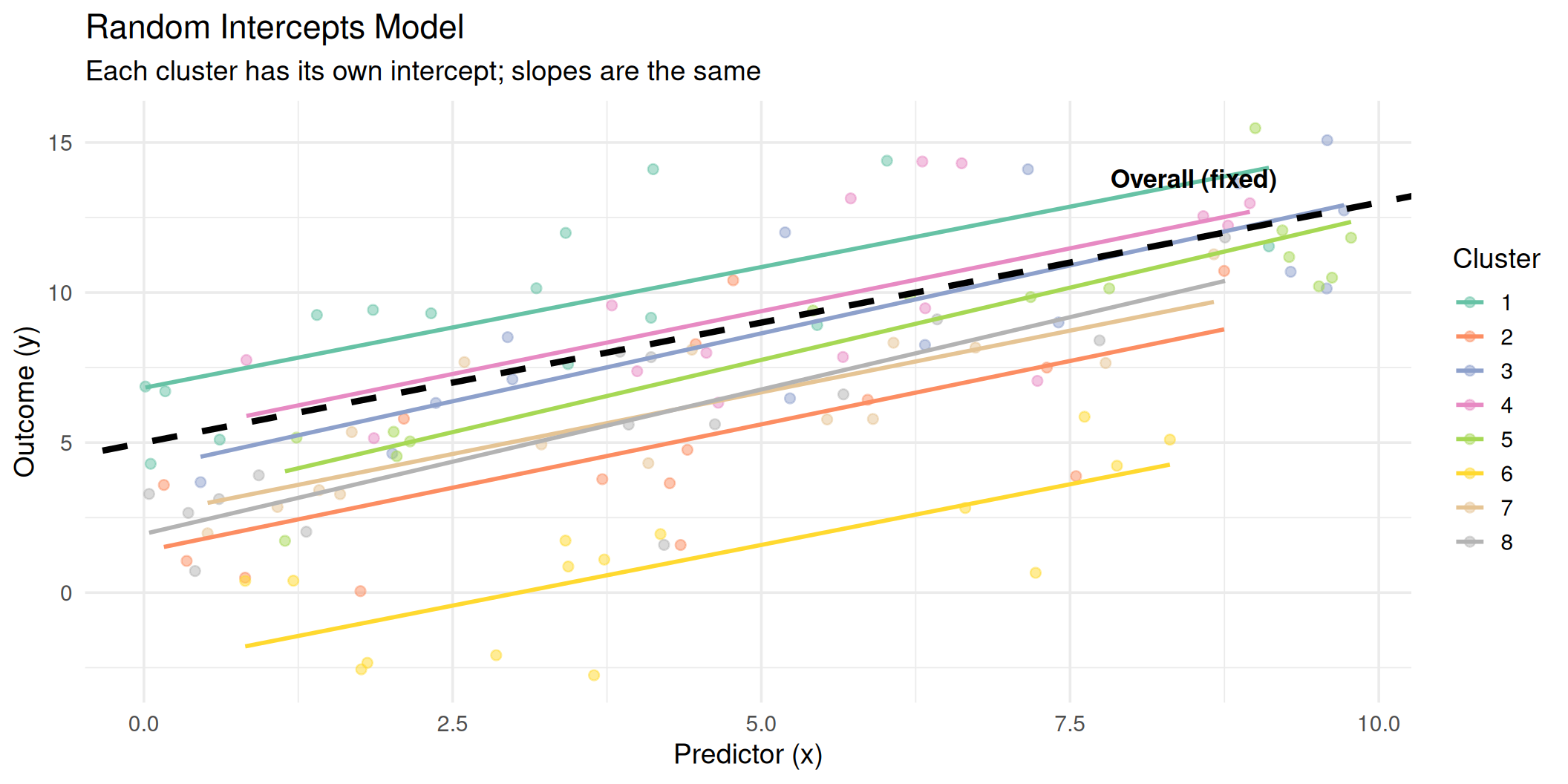
All clusters share the same slope (\(\beta_1\)), but each has its own intercept (\(\beta_0 + u_{0j}\)).
Random Slopes
We can also allow the effect of a predictor to vary across clusters:
\[y_{ij} = \beta_0 + \beta_1 x_{ij} + u_{0j} + u_{1j} x_{ij} + e_{ij}\]
where:
\[\begin{pmatrix} u_{0j} \\ u_{1j} \end{pmatrix} \sim N\left(\begin{pmatrix} 0 \\ 0 \end{pmatrix}, \begin{pmatrix} \sigma^2_{u_0} & \sigma_{u_{01}} \\ \sigma_{u_{01}} & \sigma^2_{u_1} \end{pmatrix}\right)\]
- \(u_{0j}\): cluster-specific deviation in the intercept
- \(u_{1j}\): cluster-specific deviation in the slope
- \(\sigma_{u_{01}}\): covariance between random intercept and slope
Random Slopes: Visualized
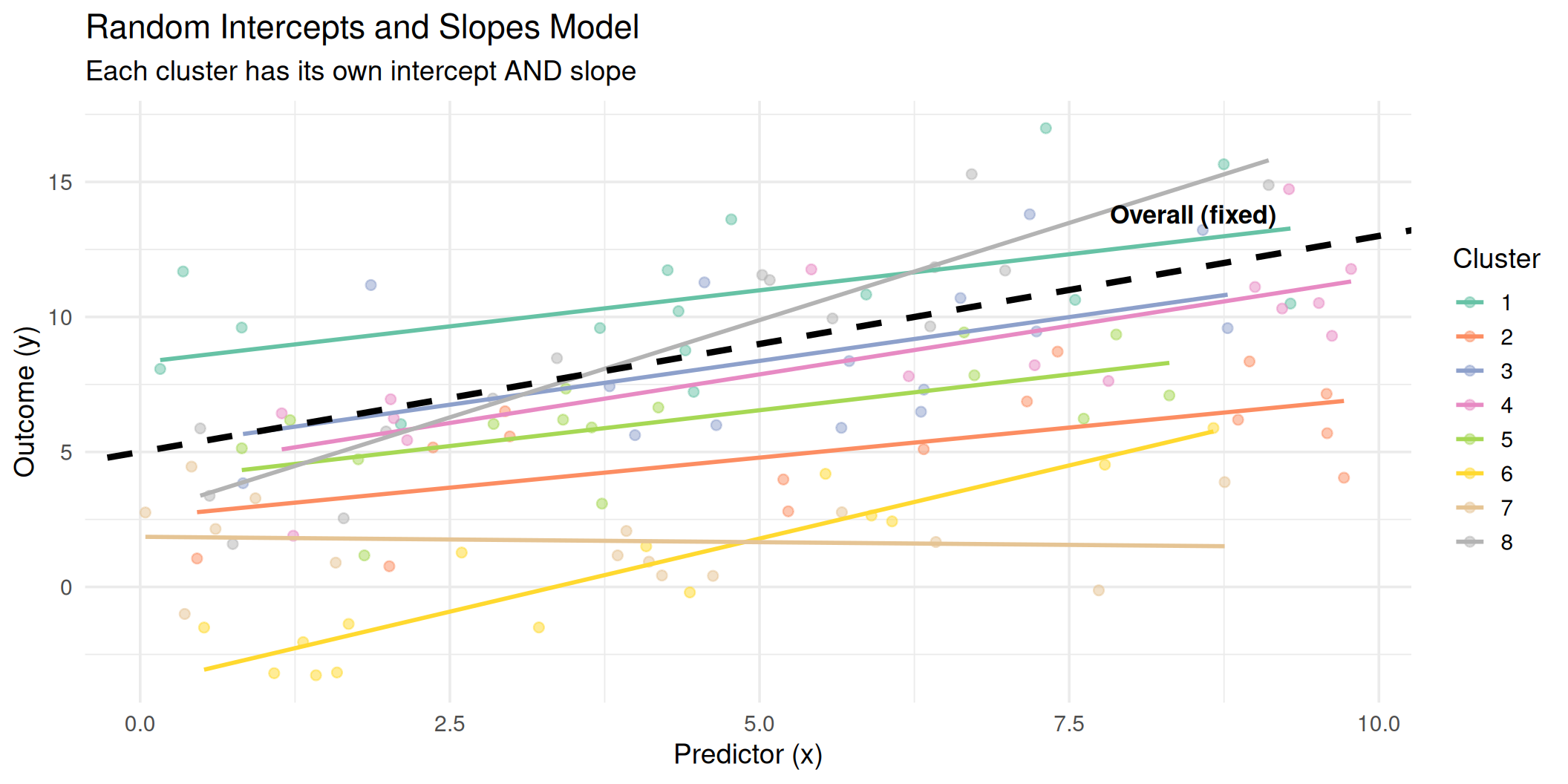
Now both the intercepts and the slopes vary across clusters. The black dashed line represents the average (fixed) relationship.
Building Up Mixed Models
| Model | Formula | Allows |
|---|---|---|
| Empty model | \(y_{ij} = \beta_0 + u_{0j} + e_{ij}\) | Decompose total variance |
| Random intercept | \(y_{ij} = \beta_0 + \beta_1 x_{ij} + u_{0j} + e_{ij}\) | Cluster-varying baselines |
| Random slope | \(y_{ij} = \beta_0 + \beta_1 x_{ij} + u_{0j} + u_{1j}x_{ij} + e_{ij}\) | Cluster-varying effects |
Typical workflow:
- Fit the empty model to estimate the ICC
- Add fixed effects (predictors)
- Test random slopes for key predictors
- Compare models using likelihood ratio tests or information criteria (AIC, BIC)
- Interpret fixed effects and variance components
Part IV: Time in Mixed Models
Longitudinal Data as Multilevel Data
Longitudinal (repeated-measures) data is a special case of multilevel data:
| Level 1 | Level 2 |
|---|---|
| Time points | Individuals |
Each person is a “cluster” of their own repeated observations. Observations within a person are correlated, which is exactly the clustering problem we discussed.
A Key Decision
In mixed models for longitudinal data, how you treat time matters enormously:
- Time as categorical: each wave gets its own mean (no functional form assumed)
- Time as continuous: assumes a specific trajectory (linear, quadratic, etc.)
This decision affects model flexibility, parsimony, and interpretation.
Time as a Categorical Variable
When time is treated as a factor (dummy-coded or effect-coded), the model estimates a separate mean for each time point:
\[y_{ij} = \beta_0 + \beta_1 D_{2ij} + \beta_2 D_{3ij} + \beta_3 D_{4ij} + u_{0j} + e_{ij}\]
where \(D_k\) are dummy variables for each time point after the first.
Advantages:
- No assumption about the shape of change
- Captures non-linear, non-monotonic patterns
- Good for designs with few, irregularly spaced waves
Disadvantages:
- Uses more degrees of freedom (\(k - 1\) parameters for \(k\) time points)
- Cannot easily extrapolate beyond observed time points
- Harder to summarize “rate of change”
- Not practical with many time points
When to Use Categorical Time
- You have \(\leq\) 5 time points
- You suspect non-linear change but don’t know the form
- The spacing between waves is uneven or the specific waves matter substantively
Time as a Continuous Variable
When time is treated as continuous, the model assumes a specific functional form for change:
Linear growth:
\[y_{ij} = \beta_0 + \beta_1 \text{time}_{ij} + u_{0j} + u_{1j}\text{time}_{ij} + e_{ij}\]
Quadratic growth:
\[y_{ij} = \beta_0 + \beta_1 \text{time}_{ij} + \beta_2 \text{time}_{ij}^2 + u_{0j} + u_{1j}\text{time}_{ij} + e_{ij}\]
Advantages:
- Parsimonious (fewer parameters)
- Interpretable rate of change (\(\beta_1\))
- Can model participants with different numbers of time points
- Handles unequally spaced observations naturally
Disadvantages:
- Assumes a specific trajectory shape
- Misspecification can bias results
When to Use Continuous Time
- You have many time points (\(\geq\) 5)
- Change is expected to be smooth
- You want to estimate individual growth trajectories
- Observations are unequally spaced
Comparing the Two Approaches
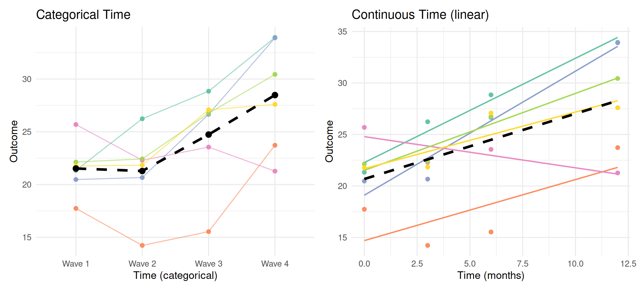
Left: No functional form assumed; each wave has its own estimated mean. Right: Linear trajectory imposed; summarized by intercept and slope.
Part V: Estimating Mixed Models in R
The lme4 Package
The workhorse for mixed-effects models in R is lme4 (with lmerTest for p-values):
The key function is lmer(), with a formula syntax that separates fixed and random effects:
| Syntax | Meaning |
|---|---|
(1 | cluster) |
Random intercept for each cluster |
(1 + x | cluster) |
Random intercept and slope for \(x\) |
(0 + x | cluster) |
Random slope only (no random intercept) |
(1 | cluster1) + (1 | cluster2) |
Crossed random effects |
Example Dataset: Sleepstudy
The sleepstudy data from lme4 tracks reaction time across 10 days of sleep deprivation in 18 subjects:
| Reaction | Days | Subject |
|---|---|---|
| 249.5600 | 0 | 308 |
| 258.7047 | 1 | 308 |
| 250.8006 | 2 | 308 |
| 321.4398 | 3 | 308 |
| 356.8519 | 4 | 308 |
| 414.6901 | 5 | 308 |
| 382.2038 | 6 | 308 |
| 290.1486 | 7 | 308 |
| 430.5853 | 8 | 308 |
| 466.3535 | 9 | 308 |
| 222.7339 | 0 | 309 |
| 205.2658 | 1 | 309 |
- Reaction: average reaction time (ms)
- Days: days of sleep deprivation (0-9)
- Subject: participant identifier (18 subjects)
Exploring the Data
ggplot(sleepstudy, aes(x = Days, y = Reaction)) +
    geom_line(aes(group = Subject), alpha = 0.3) +
    geom_point(aes(color = Subject), size = 1.5, alpha = 0.7) +
    geom_smooth(
        method = "lm",
        color = "black",
        linewidth = 1.5,
        linetype = "dashed"
    ) +
    labs(
        x = "Days of Sleep Deprivation",
        y = "Reaction Time (ms)",
        title = "Individual Trajectories of Reaction Time"
    ) +
    theme_minimal(base_size = 14) +
    theme(legend.position = "none")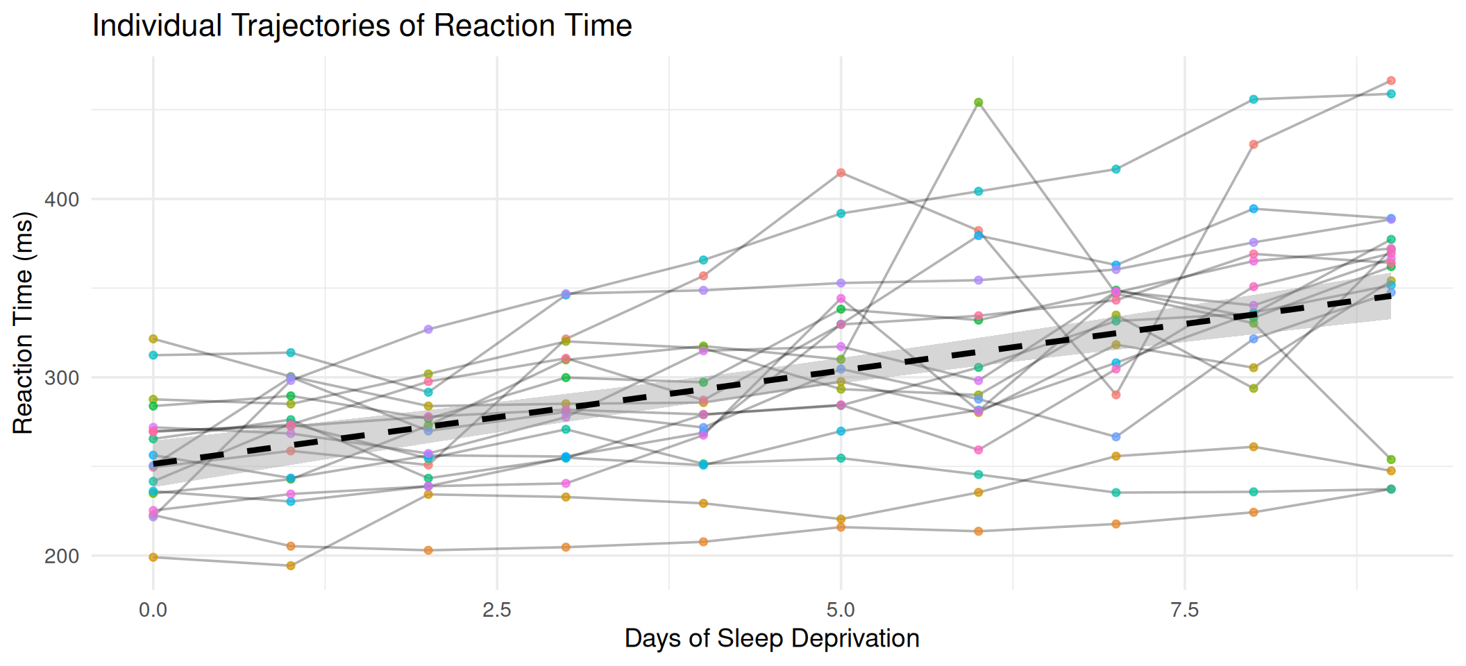
Each subject has a different baseline and a different rate of decline. A mixed model can capture both.
Step 1: The Empty Model
The empty (unconditional) model partitions total variance into between- and within-subject components:
Linear mixed model fit by REML. t-tests use Satterthwaite's method [
lmerModLmerTest]
Formula: Reaction ~ 1 + (1 | Subject)
   Data: sleepstudy

REML criterion at convergence: 1904.3

Scaled residuals:
    Min      1Q  Median      3Q     Max
-2.4983 -0.5501 -0.1476  0.5123  3.3446

Random effects:
 Groups   Name        Variance Std.Dev.
 Subject  (Intercept) 1278     35.75
 Residual             1959     44.26
Number of obs: 180, groups:  Subject, 18

Fixed effects:
            Estimate Std. Error     df t value Pr(>|t|)
(Intercept)   298.51       9.05  17.00   32.98   <2e-16 ***
---
Signif. codes:  0 '***' 0.001 '**' 0.01 '*' 0.05 '.' 0.1 ' ' 1
Computing the ICC
ICC = 0.395About 39% of the total variance in reaction time is between subjects. This justifies using a multilevel model.
Step 2: Random Intercept Model
Add Days as a fixed predictor, keeping random intercepts:
Linear mixed model fit by REML. t-tests use Satterthwaite's method [
lmerModLmerTest]
Formula: Reaction ~ Days + (1 | Subject)
   Data: sleepstudy

REML criterion at convergence: 1786.5

Scaled residuals:
    Min      1Q  Median      3Q     Max
-3.2257 -0.5529  0.0109  0.5188  4.2506

Random effects:
 Groups   Name        Variance Std.Dev.
 Subject  (Intercept) 1378.2   37.12
 Residual              960.5   30.99
Number of obs: 180, groups:  Subject, 18

Fixed effects:
            Estimate Std. Error       df t value Pr(>|t|)
(Intercept) 251.4051     9.7467  22.8102   25.79   <2e-16 ***
Days         10.4673     0.8042 161.0000   13.02   <2e-16 ***
---
Signif. codes:  0 '***' 0.001 '**' 0.01 '*' 0.05 '.' 0.1 ' ' 1

Correlation of Fixed Effects:
     (Intr)
Days -0.371
Step 3: Random Intercept and Slope
Allow the effect of Days to vary across subjects:
Linear mixed model fit by REML. t-tests use Satterthwaite's method [
lmerModLmerTest]
Formula: Reaction ~ Days + (1 + Days | Subject)
   Data: sleepstudy

REML criterion at convergence: 1743.6

Scaled residuals:
    Min      1Q  Median      3Q     Max
-3.9536 -0.4634  0.0231  0.4634  5.1793

Random effects:
 Groups   Name        Variance Std.Dev. Corr
 Subject  (Intercept) 612.10   24.741
          Days         35.07    5.922   0.07
 Residual             654.94   25.592
Number of obs: 180, groups:  Subject, 18

Fixed effects:
            Estimate Std. Error      df t value Pr(>|t|)
(Intercept)  251.405      6.825  17.000  36.838  < 2e-16 ***
Days          10.467      1.546  17.000   6.771 3.26e-06 ***
---
Signif. codes:  0 '***' 0.001 '**' 0.01 '*' 0.05 '.' 0.1 ' ' 1

Correlation of Fixed Effects:
     (Intr)
Days -0.138
Model Comparison
We use a likelihood ratio test to determine whether the random slope improves the model:
Data: sleepstudy
Models:
m1: Reaction ~ Days + (1 | Subject)
m2: Reaction ~ Days + (1 + Days | Subject)
   npar    AIC    BIC  logLik -2*log(L)  Chisq Df Pr(>Chisq)
m1    4 1802.1 1814.8 -897.04    1794.1
m2    6 1763.9 1783.1 -875.97    1751.9 42.139  2  7.072e-10 ***
---
Signif. codes:  0 '***' 0.001 '**' 0.01 '*' 0.05 '.' 0.1 ' ' 1
The significant chi-square test and lower AIC/BIC for m2 indicate that subjects differ meaningfully in how sleep deprivation affects their reaction time.
Interpreting the Results
| effect | term | estimate | std.error | statistic | df | p.value | conf.low | conf.high |
|---|---|---|---|---|---|---|---|---|
| fixed | (Intercept) | 251.41 | 6.82 | 36.84 | 17 | 0 | 237.01 | 265.80 |
| fixed | Days | 10.47 | 1.55 | 6.77 | 17 | 0 | 7.21 | 13.73 |
Fixed effects:
- Intercept (\(\hat{\beta}_0\) = 251.4 ms): average reaction time at Day 0
- Days (\(\hat{\beta}_1\) = 10.5 ms/day): average increase in reaction time per additional day of sleep deprivation
Random effects:
| effect | group | term | estimate |
|---|---|---|---|
| ran_pars | Subject | sd__(Intercept) | 24.74 |
| ran_pars | Subject | sd__Days | 5.92 |
| ran_pars | Subject | cor__(Intercept).Days | 0.07 |
| ran_pars | Residual | sd__Observation | 25.59 |
Subjects vary in both their baseline reaction time and in how much sleep deprivation affects them.
Visualizing Model Predictions
sleepstudy$pred <- predict(m2)

ggplot(sleepstudy, aes(x = Days, y = Reaction)) +
    geom_point(alpha = 0.4) +
    geom_line(aes(y = pred, color = Subject), linewidth = 0.8) +
    geom_abline(
        intercept = fixef(m2)[1],
        slope = fixef(m2)[2],
        linewidth = 1.5,
        linetype = "dashed"
    ) +
    labs(
        x = "Days of Sleep Deprivation",
        y = "Reaction Time (ms)",
        title = "Subject-Specific Predictions from the Random Slopes Model",
        subtitle = "Dashed line = population average (fixed effects)"
    ) +
    theme_minimal(base_size = 14) +
    theme(legend.position = "none")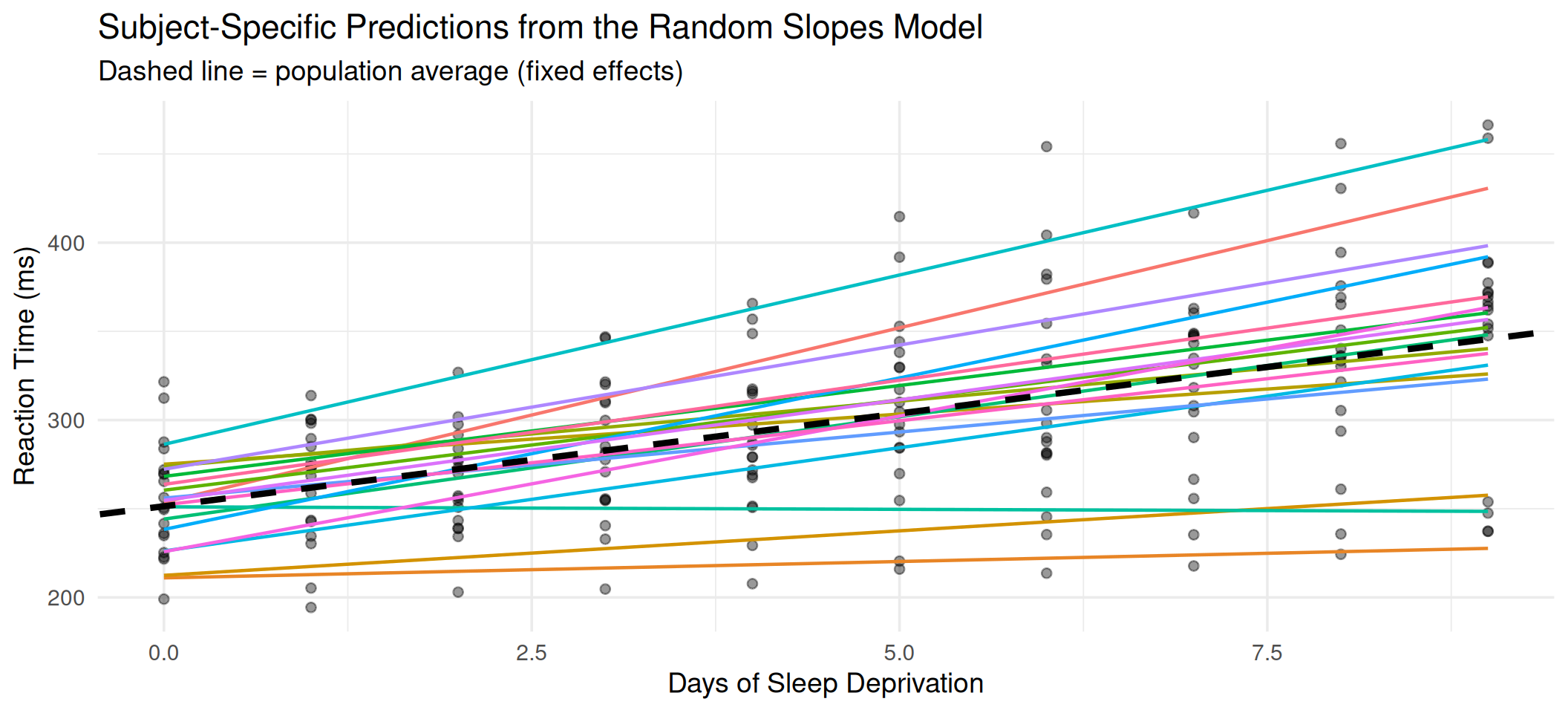
Categorical vs. Continuous Time: Sleepstudy
Let’s compare both approaches on the same data:
Continuous time (linear):
(Intercept)        Days
     251.41       10.47
2 fixed-effect parameters.
Categorical time:
(Intercept)   Days_cat1   Days_cat2   Days_cat3   Days_cat4   Days_cat5
     256.65        7.84        8.71       26.34       32.00       51.87
  Days_cat6   Days_cat7   Days_cat8   Days_cat9
      55.53       62.10       79.98       94.20
10 fixed-effect parameters (reference + 9 dummies).
Comparing Fits
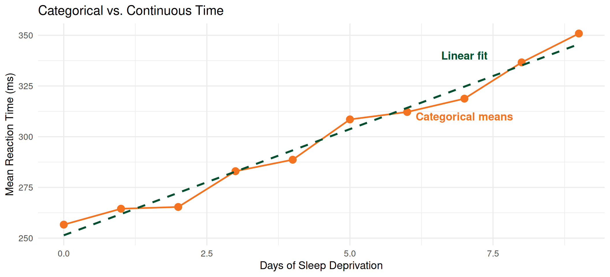
In this case, the linear model provides a good approximation. But when trajectories are non-linear, categorical time will better capture the actual pattern of change.
Part VI: Generalized Estimating Equations (GEE)
Mixed Models vs. GEE: Two Philosophies
Mixed-effects models (subject-specific):
- Model the individual trajectories
- Random effects capture within-cluster correlation
- Coefficients are conditional on the random effects
- “How does \(x\) affect \(y\) for a given individual?”
- Requires distributional assumptions about random effects (\(u_j \sim N(0, \sigma^2_u)\))
GEE (population-averaged):
- Model the marginal (population-level) mean
- Working correlation structure accounts for clustering
- Coefficients are marginal, averaged over all clusters
- “How does \(x\) affect the average \(y\) in the population?”
- No distributional assumptions about random effects
- Uses sandwich (robust) standard errors for valid inference
Important
For linear models with identity link, mixed-effects and GEE often give similar fixed-effect estimates. The differences become substantial for non-linear models (logistic, Poisson).
When Does GEE Shine?
Use GEE when:
- You care about population-averaged effects, not individual trajectories
- You have non-linear outcomes (binary, count) where the conditional vs. marginal distinction matters
- You want robustness to misspecification of the correlation structure
- You don’t need to predict individual outcomes
- Your focus is on public health or policy implications (e.g., “What happens on average if we intervene?”)
Stick with mixed models when:
- You need individual-level predictions (BLUPs)
- You want to estimate the variance of individual differences
- Your research question is about individual trajectories
- You have unbalanced data with informative dropout (GEE assumes MCAR for dropout)
- You need to model complex random-effects structures
An Important Limitation of GEE
Standard GEE assumes that missing data is MCAR. If dropout is related to observed data (MAR), weighted GEE or mixed models are preferable.
The GEE Framework
GEE specifies three components:
- Mean model (same as GLM):
\[E[y_{ij}] = g^{-1}(\beta_0 + \beta_1 x_{ij})\]
Working correlation structure: an assumed form for the within-cluster correlations (does not need to be exactly correct)
Sandwich estimator: robust standard errors that are valid even if the working correlation is wrong
| Working Correlation | Assumes | Best For |
|---|---|---|
| Independence | No within-cluster correlation | Baseline; always valid with sandwich SE |
| Exchangeable | Constant correlation within clusters | Cross-sectional clusters (schools, clinics) |
| AR(1) | Correlation decays with time lag | Equally spaced longitudinal data |
| Unstructured | No restrictions | Few time points; most flexible |
GEE in R: The geepack Package
Call:
geeglm(formula = Reaction ~ Days, data = sleepstudy, id = Subject,
    corstr = "exchangeable")

 Coefficients:
            Estimate Std.err    Wald Pr(>|W|)
(Intercept)  251.405   6.632 1436.89  < 2e-16 ***
Days          10.467   1.502   48.55 3.22e-12 ***
---
Signif. codes:  0 '***' 0.001 '**' 0.01 '*' 0.05 '.' 0.1 ' ' 1

Correlation structure = exchangeable
Estimated Scale Parameters:

            Estimate Std.err
(Intercept)     2251   536.6
  Link = identity

Estimated Correlation Parameters:
      Estimate Std.err
alpha    0.576  0.1114
Number of clusters:   18  Maximum cluster size: 10
Comparing GEE and Mixed Model Estimates
| term | estimate | std.error | Method |
|---|---|---|---|
| (Intercept) | 251.41 | 6.82 | Mixed Model (lmer) |
| Days | 10.47 | 1.55 | Mixed Model (lmer) |
| (Intercept) | 251.41 | 6.63 | GEE (exchangeable) |
| Days | 10.47 | 1.50 | GEE (exchangeable) |
For this linear model with a continuous outcome, the fixed-effect estimates are very similar. The differences would be more pronounced with binary or count outcomes.
GEE with Different Correlation Structures
| Correlation | estimate | std.error | p.value |
|---|---|---|---|
| Independence | 10.47 | 1.502 | 0 |
| Exchangeable | 10.47 | 1.502 | 0 |
| AR(1) | 10.47 | 1.448 | 0 |
The point estimates are nearly identical across correlation structures. The standard errors differ slightly, but the sandwich estimator provides robustness.
When Conditional \(\neq\) Marginal
For linear models:
\[E[y_{ij} | u_j] = \beta_0 + \beta_1 x_{ij} + u_j\]
Marginalizing over \(u_j\):
\[E[y_{ij}] = \beta_0 + \beta_1 x_{ij}\]
The fixed effects are the same; linear models “collapse” nicely.
For logistic models:
\[\text{logit}(P(y_{ij} = 1 | u_j)) = \beta_0 + \beta_1 x_{ij} + u_j\]
Marginalizing over \(u_j\):
\[\text{logit}(P(y_{ij} = 1)) \neq \beta_0 + \beta_1 x_{ij}\]
The marginal coefficients are attenuated relative to conditional coefficients. The GEE estimates are closer to zero than the GLMM estimates.
Rule of Thumb
For logistic models, the marginal (GEE) coefficient \(\approx \beta_{\text{conditional}} / \sqrt{1 + c^2 \sigma^2_u}\) where \(c \approx 16\sqrt{3}/(15\pi)\).
Summary: Mixed Models vs. GEE
| Feature | Mixed-Effects Model | GEE |
|---|---|---|
| Coefficients | Subject-specific (conditional) | Population-averaged (marginal) |
| Random effects | Explicitly modeled | Not modeled (nuisance) |
| Correlation | Implied by random effects | Specified by working correlation |
| Robustness | Sensitive to RE distribution | Robust via sandwich SE |
| Missing data | Valid under MAR | Valid under MCAR (standard GEE) |
| Individual predictions | Yes (BLUPs) | No |
| Non-linear outcomes | Conditional estimates | Marginal estimates |
| Best for | Individual trajectories, prediction | Population effects, policy questions |
Choosing Between the Two
Ask yourself:
- Am I interested in what happens to the average person in the population, or in individual variation?
- Population average → GEE
- Individual variation → Mixed model
- Is my outcome continuous or binary/count?
- Continuous → Often similar results
- Binary/Count → Results differ; choose based on Q1
- Do I suspect informative dropout?
- Yes → Mixed model (valid under MAR)
- No or MCAR → Either approach works
Practical Recommendation
In many applications, it is informative to fit both and compare. If results are similar, the conclusions are robust. If they differ, understanding why they differ provides insight into the data structure.
Wrapping Up
Key Takeaways
Independence matters: Classical methods assume independent observations. Violating this inflates Type I error.
Clustered data is everywhere: Students in schools, patients in clinics, repeated measures, all create dependencies.
Mixed-effects models handle clustering by modeling between-cluster variation with random effects.
Time can be categorical or continuous: Categorical time is flexible but costly in parameters; continuous time is parsimonious but assumes a functional form.
GEE offers an alternative that focuses on population-averaged effects with robust standard errors.
The choice between mixed models and GEE depends on your research question: individual trajectories vs. population effects.
References
- Raudenbush, S. W., & Bryk, A. S. (2002). Hierarchical Linear Models (2nd ed.). Sage.
- Snijders, T. A. B., & Bosker, R. J. (2012). Multilevel Analysis (2nd ed.). Sage.
- Fitzmaurice, G. M., Laird, N. M., & Ware, J. H. (2011). Applied Longitudinal Analysis (2nd ed.). Wiley.
- Liang, K.-Y., & Zeger, S. L. (1986). Longitudinal data analysis using generalized linear models. Biometrika, 73(1), 13–22.
- Bates, D., Maechler, M., Bolker, B., & Walker, S. (2015). Fitting linear mixed-effects models using lme4. Journal of Statistical Software, 67(1), 1–48.
- Enders, C. K., & Tofighi, D. (2007). Centering predictor variables in cross-sectional multilevel models. Psychological Methods, 12(2), 121–138.
Questions?

EPH 752 Advanced Research Methods