Computing Sensitivity and Specificity Using collect_metrics
Sensitivity
Tidymodels
Specificity
Authors
Francisco Cardozo
Catalina Cañizares
Published
July 22, 2023
(in progress)
In the last post, we discussed computing sensitivity and specificity using the sensitivity() and specificity() functions from the yardstick package. In this post, we’ll demonstrate how to compute these metrics using the collect_metrics function from the tidymodels package.
Dataset
First, let’s recreate the confusion matrix from the previous post.
The tbl_cross() function is useful for computing these metrics after a bit of data wrangling.
# Duplicate each row of the tibble based on the value in the Count columnconfusion_matrix_long |>uncount(Count) |>tbl_cross(percent ="col")
True Class
Total
True 0
True 1
Predicted Class
0
35 (70%)
10 (20%)
45 (45%)
1
15 (30%)
40 (80%)
55 (55%)
Total
50 (100%)
50 (100%)
100 (100%)
The sensitivity of our model is 80%, and the specificity is 70% - pretty good values!
Computing Sensitivity and Specificity Using collect_metrics
In machine learning, sensitivity and specificity are important metrics used to evaluate and improve model performance. When we tune model parameters across different datasets, it’s useful to compute these metrics for each dataset. This gives us useful data to make decisions on enhancing model performance. We can calculate these metrics efficiently using the collect_metrics() function from the tidymodels package.
We’ll use fit_resamples() to estimate the model many times. This uses different samples from our training data. Then, we’ll use collect_metrics() to compute the sensitivity and specificity for each dataset.
Cross-Validation Folds
We’ll start by using vfold_cv() from tidymodels to create 10 folds of data. To get a better estimate of the sensitivity and specificity, we’ll use the repeats argument to repeat the sampling process 10 times. This gives us 100 folds of data in total.
# Load packageslibrary(tidymodels) # Load tidymodels packagetidymodels::tidymodels_prefer() # Set tidymodels as the default modeling frameworkset.seed(1906) # Set seed for reproducibility# Create a tibble with the datadf <- confusion_matrix_long |>uncount(Count) |>rename(x =`Predicted Class`, y =`True Class` )# Create 10 folds of the datafolds <-vfold_cv(df, v =10, repeats =10)
Model Specification
Having the folds ready, we can now specify the model.
# Define a logistic regression model specificationmodel_spec <-logistic_reg() |>set_engine("glm") |>set_mode("classification")# Create a recipe for preprocessing the datarecipe_glm <-recipe(y ~ x, data = df) |># Convert all nominal variables to dummy variablesstep_dummy(all_nominal(), -all_outcomes()) # Define a workflow for fitting the logistic regression modelwr_glm <-workflow() |># Add the recipe to the workflowadd_recipe(recipe_glm) |># Add the model specification to the workflowadd_model(model_spec)
Perfect! Now we are ready to estimate the model.
Estimating the Model
# Estimate the model 100 timesmodel_resamples <-fit_resamples( wr_glm, folds, control =control_resamples(save_pred =TRUE))
Notice that we used the save_pred argument in control_resample() because we want to save the predictions of the model for each fold. This allows us to compute the sensitivity and specificity for each fold, which is the goal of this post.
Let’s take a look at one of the results.
# Extract the metrics for the first resamplemodel_resamples |># Select the first resampleslice(1) |># Unnest the metrics dataunnest(.metrics) |>select(.metric, .estimate) |>gt() |>fmt_number(decimals =3)
.metric
.estimate
accuracy
0.700
roc_auc
0.786
By default, we obtain accuracy and roc_auc metrics for classification models. However, we want a specific metric set (sensitivy and specificity). To achieve this, we can use metric_set() function from the yardstick package.
Cautionevent_level = ?
Be mindful of the event level used by yardstick. As we demonstrated in the previous post, yardstick uses the first level as the event of interest. To change this behavior, we need to specify the event_level argument when using the fit_resamples() function.
Computing Sensitivity and Specificity
# Define the metrics to usemy_metrics <-metric_set(sens, spec)# Fit the logistic regression model using resamplingmodel_resamples <-fit_resamples( wr_glm, folds, metrics = my_metrics,control =control_resamples(# Save the predicted values for each resamplesave_pred =TRUE,# Set the event level to "second"event_level ="second" ))
Tip
You can find all available metrics in yardstick here.
Now, let’s dive into the results. For a start, we’ll focus on the first resample. Although this may provide an imperfect estimation of our “true” values, theory assures us that as we increase the number of resamples, the average of the metrics will move closer to these “true” values. Let’s see this in action!
# Extract the metrics for the first resamplemodel_resamples %>%# Select the first resampleslice(1) %>%# Unnest the metrics dataunnest(.metrics) %>%# Select the metric and estimate columnsselect(.metric, .estimate) %>%# Create a gt tablegt() %>%# Format the estimate column to 3 decimal placesfmt_number(decimals =3)
.metric
.estimate
sens
1.000
spec
0.571
Good, we have achieved a sensitivity of 100% and specificity of 57.1%, which, frankly, isn’t an ideal representation of our true values. But, let’s keep in mind, this is just a single estimate out of our 100 trials. Now, let’s take it to the next level and summarize these values across all our estimates.
# Collect and summarise the metrics for all resamplesmodel_resamples %>%# Collect the metrics and summarise themcollect_metrics(summarise =TRUE) %>%# Create a gt tablegt() %>%# Format the table to 3 decimal placesfmt_number(decimals =3)
.metric
.estimator
mean
n
std_err
.config
sens
binary
0.810
99.000
0.017
Preprocessor1_Model1
spec
binary
0.703
100.000
0.018
Preprocessor1_Model1
Great job! Our model’s estimated sensitivity is at 81.0% and specificity stands at 70.3%, quite near to our actual values.
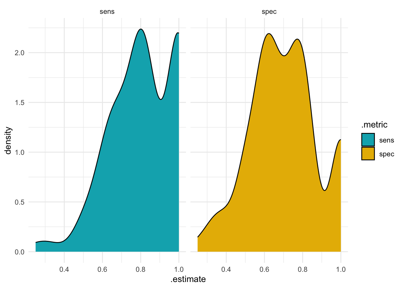
With all this valuable data at hand, it’s tempting to visualize it. So, let’s move on to plotting the observed distribution for both sensitivity and specificity values to get a better understanding of our model’s performance.
Next time, we’ll look more closely at these values. We’ll work out which ones are bigger than 0.5 and see how spread out they are. But, we need to be careful because these numbers are connected; they all come from the same data. Don’t miss it!
Summary
In this blog post, we discussed the use of the tidymodels package to compute the sensitivity and specificity of a model - two important measures for evaluating model performance. We started with the recreation of a confusion matrix, then used the tbl_cross() function to perform some data wrangling.
Next, we leveraged fit_resamples() from the tidymodels package to estimate our model multiple times, using cross-validation with 10 repeated folds to create 100 datasets in total.
We set up a logistic regression model, fit it to our data, and estimated the model multiple times using the created folds. The saved predictions allowed us to compute sensitivity and specificity for each fold.
We defined a custom set of metrics - roc_auc, sensitivity, and specificity - using the metric_set() function from the yardstick package. Finally, we used collect_metrics() to compute the average of these metrics for all the folds, and visualized the distribution of the sensitivity and specificity values.
Future posts will delve into calculating confidence intervals and evaluating the variability of these values across resamples.