Machine Learning for Public Health
July 30, 2024
The Importance of Prediction in Public Health
What are the underlying causes of a health problem? For example, what are the causes of youth alcohol initiation?
What are the risk factors associated with a health problem? Which demographic and behavioral factors increase the likelihood of developing type 2 diabetes among adults?
- Can we predict the future appearance of a health problem? Can we forecast the potential outbreak of seasonal influenza in the upcoming months?

Regularization
- Technique to prevent overfitting.
- Controls the complexity of the model.
- Adds some bias to the model to reduce variance.

Bias-variance Trade-off
Bias: Error due to overly simplistic assumptions. Variance: Error due to overly complex models. The goal is to minimize the total error.

Simulation Example
Estimate these models in a few cases. Then progressively increase the sample size by one unit. Calculate the training and testing errors each time.

First Scenario
A linear problem - linear regression.
Second Scenario
Non-linear problem - linear regression.

Third Scenario
Non-linear problem - Support Vector Machine.
Fourth Scenario
A linear problem - Random Forest.

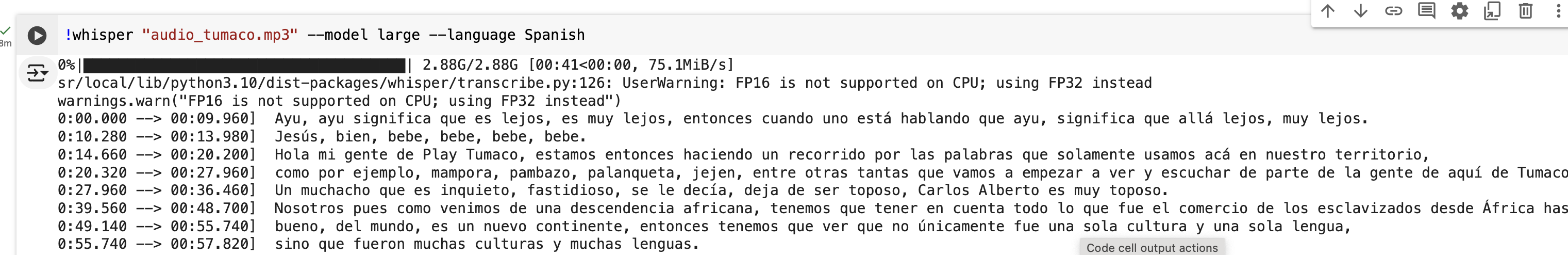
Transformers
Audio

Audio
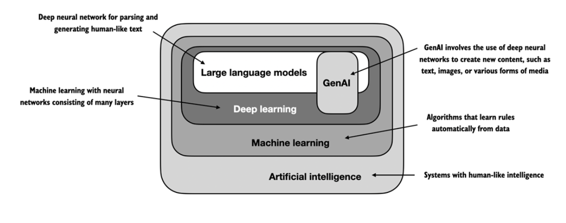
What are Large Language Models?
- Something that knows how to predict the next word in a sentence or fill in the missing words in a sentence.
- Large language models (LLMs) are a type of artificial intelligence that can generate human-like text.
- They are trained on vast amounts of text data.
What can you do with LLMs?
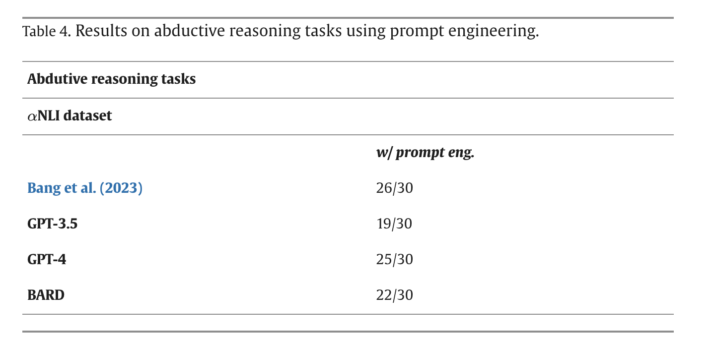
- Prompt and RAG the models (López Espejel et al. 2023)
![]()

Prompt and RAG the models

Prompt and RAG the models
What can you do with LLMs?
- Study, optimize, and debug the models
- Agents (Park et al. 2023; Kapoor et al. 2024)

Ethical Dilemmas

- Bias, fairness, security, privacy, transparency, accountability, and trust.
- The potential for misuse of large language models is a major concern.
- How people apply moral and ethical principles to the development and use of large language models is a critical issue.
- How people reason in terms of accountability when interacting with large language models.